Effective and Efficient Pruning of Meta-Classifiers in a Distributed Data Mining System ∗ Andreas L. Prodromidis †
Salvatore J. Stolfo
Philip K. Chan
Computer Science Department Columbia University New York, NY 10027
[email protected]
Computer Science Department Columbia University New York, NY 10027
[email protected]
Computer Science Department Florida Institute of Technology Melbourne, FL 32901
[email protected]
July 31, 1998
Abstract Distributed data mining systems aim to discover and combine useful information that is distributed across multiple databases. One of the main challenges is the design of effective and efficient methods to combine multiple models computed over multiple distributed sources that scale well over many large distributed databases. We describe in detail several methods that evaluate, prune and combine large collections of imported models computed at remote sites into efficient and scalable meta-classifiers. We demonstrate and evaluate the pruning methods by detailing many experiments performed on actual credit card data sets supplied by collaborating financial institutions, where the target learning task is fraud detection. We show that pruned meta-classifiers can sustain or even improve predictive performance at a substantially higher throughput, compared to the unpruned meta-classifiers. Keywords: distributed data mining, meta-learning, classifier evaluation, pruning, ensembles of classifiers, machine learning, credit card fraud detection. Contact Author: Andreas Prodromidis (Tel: 212-939-7078, Fax: 212-666-0140, e-mail:
[email protected])
∗
This research is supported by the Intrusion Detection Program (BAA9603) from DARPA (F30602-96-1-0311),
NSF (IRI-96-32225 and CDA-96-25374) and NYSSTF (423115-445). † Supported in part by an IBM fellowship
1 Introduction Machine learning constitutes a significant part in the overall Knowledge Discovery and Data Mining (KDD) process, the process of extracting useful knowledge from large databases. One means of analyzing and mining useful information from large databases is to apply various machine learning algorithms to discover patterns exhibited in the data and compute descriptive representations (also called classifiers or models) that can be subsequently used for a variety of strategic and tactical purposes. Machine learning or inductive learning (or learning from examples [23]) aims to identify regularities in a given set of training examples with little or no knowledge about the domain from which the examples are drawn. Given a set of training examples, i.e. {(x1 , y1), ..., (xn , yn )}, for some unknown function y = f (x), each interpreted as a set of attribute (feature) vectors x of the form {x1 , x2 , ..., xm } and a class label y associated with each vector, y ∈ {y 1 , y 2, ..., y k }, the task is to compute a classifier or model fˆ that approximates f and correctly labels any feature vector drawn from the same source as the training set, for which the class label y is unknown. Some of the common representations used for the generated classifiers are decision trees, rules, version spaces, neural networks, distance functions, and probability distributions. In general, these representations are associated with different types of algorithms that extract different types of information from the database and provide alternative capabilities besides the common ability to classify unknown instances drawn from some domain. However, one of the main challenges in knowledge discovery and data mining is the development of inductive learning techniques that scale up to large and (physically) distributed data sets. Many organizations seeking added value from their data are already dealing with overwhelming amounts of information that in time will likely grow in size faster than available improvements in machine resources. Many of the current generation of learning algorithms are computationally complex and require all the data to be resident in main memory which is clearly untenable for many realistic problems and databases. Furthermore, in certain cases, the data may be inherently distributed and cannot be localized on any one machine (even by a trusted third party) for a variety of practical reasons including physically dispersed mobile platforms like an armada of ships, security and fault tolerant distribution of data and services, competitive (business) reasons, as well as statutory constraints imposed by law. In such situations, it may not be possible, nor feasible, to inspect all of the data at one processing site to compute one primary “global” classifier or model at a
1
reasonable cost. We call the problem of learning useful new information from large and inherently distributed databases, the scaling problem for machine learning. Meta-learning [8], a technique similar to stacking [40], was developed recently to deal with the scaling problem. The basic idea is to execute a number of machine learning processes on a number of data subsets in parallel, and then to combine their collective results (classifiers) through an additional phase of learning. Initially, each machine learning task, also called a base learner, computes a base classifier, i.e. a model of its underlying data subset or training set. Next, a separate machine learning task, called a meta-learner, integrates these independently computed base classifiers into a higher level classifier, called a meta classifier, by learning over a meta-level training set. This meta-level training set is composed from the predictions of the individual base classifiers when tested against a separate subset of the training data, also called a validation set. From these predictions, the meta-learner discovers the characteristics and performance of the base classifiers and computes a meta-classifier which is a model of the “global” data set. To classify an unlabeled instance, the base classifiers present their own predictions to the meta-classifier which then makes the final classification. Meta-learning addresses the scaling problem for machine learning. It improves efficiency by executing in parallel the base-learning processes (implemented as a distinct serial program) on (possibly disjoint) subsets of the training data set (a data reduction technique). This approach has the advantage, of using serial code (without the time-consuming process of parallelizing it) and applying such code on small subsets of data that fit in main memory. Meta-learning, is scalable because meta-classifiers are classifiers themselves that can be further combined into higher level meta-classifiers in a bottom-up and distributed fashion. Furthermore, it improves accuracy by combining different learning systems each having different inductive bias (e.g representation, search heuristics, search space) [25]. By combining separately classifiers, meta-learning is expected to derive a higher level learned model that explains a large database more accurately than any of the individual learners. The JAM system (Java Agents for Meta-learning) [38] is a distributed agent-based data mining system that implements meta-learning. JAM takes full advantage of the inherent parallelism and distributed nature of meta-learning by providing a set of learning agents that compute models (classifier agents) over data stored locally at a site, by supporting the remote dispatch and exchange of learning and classifier agents among the participating data base sites through a special distribution mechanism, and by providing a set of meta-learning agents that combine the computed models 2
that were learned (perhaps) at different sites. There are several desiderata for a distributed data mining system. It must be: extensible, to allow use of past, present of future learning algorithm; portable, to be able to operate across different environments, e.g across the internet; scalable, to deal effectively with increasing number of data sites and database sizes; efficient, to utilize effectively the available system resources; adaptive, to be able to incorporate new information as it becomes available; compatible, to be able to integrate information from similar databases but of different schemas, and last but not least, effective, to generate accurate models of the underlying databases. It will not be possible to cover all these issues in this paper. The extensibility and portability issues are described in detail in [38], and adaptivity is discussed in [29]. Compatibility is attained by several techniques that allow distributed data mining systems to cope with incompatible classifiers, i.e. classifiers that are trained from databases with similar but not identical schemas, presented in detail in [28]. Here, we concentrate on the scalability and efficiency of distributed data mining systems. The goal is dual: 1. to acquire and combine information from multiple databases in a timely manner and 2. to generate efficient meta-classifiers. We address these two issues by employing meta-learning as a distributed learning method. Then we introduce distributed management protocols among the data sites that provide for the exchange of classifiers among remote sites. We then describe fast methods to evaluate these classifiers, filtering out (pruning) redundant models and deploying only the most essential classifiers to prevent the formation of complex, large and inefficient meta-classifiers. Through experiments performed on real credit card data provided by two different financial institutions, we evaluate the effectiveness of the proposed methods, we expose their limitations and dependencies to the particular data mining problem and we demonstrate that JAM, when provided with certain pruning methods, has the potential to improve efficiency without sacrificing predictive performance. The remainder of this paper is organized as follows: Section 2 describes the problem in detail and outlines our approach. Section 3 and 4 describe two different methods on pruning metaclassifiers. In Section 5 we present the experiments performed and the performance results collected and Section 6 concludes the paper.
3
2 Performance of Distributed Data Mining Systems Distributed data mining systems are compared with respect to their efficiency and scalability and with respect to the accuracy of their results. This section describes our approach from both perspectives.
2.1 Efficiency and Scalability The main challenge in data mining and machine learning is to deal with large problems in a “reasonable” amount of time and at an acceptable cost. To our knowledge, JAM is the only data mining system to date that employs meta-learning as a means to mine distributed databases. However, the literature reports an extensive collection of methods that facilitate the use of inductive learning algorithms for mining very large databases [10]. Provost and Kolluri [32] categorized the available methods into three main groups; methods that rely on the design of fast algorithms, methods that reduce the problem size by partitioning the data and methods that employ a relational representation. Meta learning can be considered primarily as a method that reduces the size of the data, basically due to its data reduction technique and its parallel nature. On the other hand, it is also generic, meaning that it is algorithm and representation independent, hence it can benefit from fast algorithms and efficient relational representations. Distributed systems have an additional level of complexity compared to serial, host-based systems. Distributed systems may need to deal with possibly heterogenous platforms, with several databases with (possibly) different schemas, with the design and implementation of scalable and effective protocols and with the selective and efficient use of the information gathered from the peer data sites. The scalability of a data mining system depends on the protocols that allow the collaboration and transfer of information among the data sites while efficiency relies on the appropriate evaluation and filtering of the total available set of models to minimize redundant use of system resources. One of the most significant problems for the design of a distributed data mining system is to combine scalability and efficiency without sacrificing accuracy performance. To understand the issues and tackle the complexity of the problem, we examine scalability and efficiency at two levels, the system architecture level and the meta-learning level. In the first case, we focus on the components of the system and its overall architecture. Assuming that the data mining system comprises several data sites, each with its own resources, databases, 4
machine learning agents and meta-learning capabilities, the problem is to design a protocol that would allow the data sites to collaborate efficiently without hindering their progress. Our goal is to allow the data sites to operate either independently or in collaboration without depending upon or being controlled by other “manager” sites. The protocol in a distributed data mining system should support dynamic reconfiguration of the system architecture (in case more data sites become available) and it should be scalable to allow data sites to participate in large numbers. Asynchronous protocols avoid the overheads of synchronization points introduced by synchronous protocols even though synchronous protocols are simpler and easier to design and implement. JAM has been designed around asynchronous protocols. Briefly, the JAM system can be viewed as a coarse-grain parallel application where the constituent sites function autonomously and (occasionally) exchange classifiers with each other. JAM is designed with asynchronous, distributed communication protocols that enable the participating database sites to operate independently and collaborate with other peer sites as necessary, thus eliminating centralized control and synchronization points. Employing efficient distributed protocols addresses the scalability problem only partially. The analysis of the dependencies among the classifiers and the management of the agents within the data sites constitutes the other half of the scalability problem. If not controlled properly, the size and arrangement of the classifiers inside each data site may incur unnecessary and prohibitive overheads. Meta-classifiers are defined recursively as collections of classifiers structured in multilevel trees. Being hierarchically structured, meta-classifiers can promote scalability and efficiency in a simple and straight forward manner. It is possible, however, that certain conditions yield the opposite effects. As the number of data sites, the size of data subsets and the number of deployed learning algorithms increases, more base classifiers are made available to each site and meta-learning and meta-classifying are bound to strain system resources. To make things worse, meta-classifier trees can be re-built, and grown in breadth and depth as new information and new classifiers become available. Hence, in the second case, we delve inside the data sites to explore the types, characteristics and properties of the classifiers that participate in the distributed computation. We investigate the effects of pruning and discarding certain base-classifiers on the performance of the meta-classifier. From actual experiments on base- and meta-classifiers trained to detect credit card fraud, we measured, a decrease of 50%, 90% and 95% in throughput for meta-classifiers composed of 13, 60 and 100 base-classifiers respectively.1 As more base-classifiers are combined in a 1
The experiments were conducted on a Personal Computer with a 200MHz Pentium processor running Solaris
2.5.1. Throughput here means the rate at which a stream of data items can be piped through and labeled by a meta-
5
meta-classifier, additional time and resources are required to classify new instances and that translates to increased overheads and lower throughputs. Memory constraints are equally important. For the same problem, a single ID3 decision tree ([33]) may require more than 750KBytes of main memory, while a C4.5 decision tree ([34]) may need 80KBytes. Retaining a large number of base classifiers and meta-classifiers may not be practical nor feasible. The objective of pruning is to build partially grown meta-classifiers (meta-classifiers with pruned subtrees) to achieve comparable or better performance (accuracy) resul ts than fully grown meta-classifiers. Pre-training pruning refers to the filtering of the classifiers before they are used in the training of a meta-classifier. Instead of combining classifiers in a brute force manner, with pre-training pruning we introduce a preliminary stage for analyzing the available classifiers and qualifying them for inclusion in a meta-classifier. Only those classifiers that appear (according to one or more pre-defined metrics) to be most “promising” participate in the final meta-classifier. Conversely, post-training pruning, denotes the evaluation and pruning of constituent base classifiers after a complete meta-classifier has been constructed.
2.2 Effectiveness We seek effective measures to compare local and imported classifiers that are fast to compute and that choose the “best” classifiers to combine so that other classifiers can be discarded. Ideally, the resulting combined ensemble of classifiers should produce a smaller, less expensive meta-classifier with the best possible performance (from the perspective of predictive accuracy and/or cost). For example, many combining techniques (that have been proposed) aim to maximize the accuracy of the ensemble. We consider alternative “optimality criteria”. We seek to minimize the computational expense of the ensemble meta-classifier while maximizing its predictive efficacy. Predictive efficacy does not mean only overall accuracy (or minimal error). Other measures of interest include True Positive (TP) and False Positive (FP) rates for binary classification problems, ROC analysis and problem specific cost models are all different criteria relevant to different problems and learning tasks. In the credit card fraud domain, for example, overall predictive accuracy is inappropriate as the single measure of predictive performance. If 1% of the transactions are fraudulent, then a model that always predicts “non-fraud” will be 99% accurate. Hence, TP rate is more important. Of the 1% fraudulent transactions, we wish to compute models that predict 100% of these, yet classifier, as for example, in real-time fraud detection of a stream of transactions.
6
produce no false alarms (i.e. predict no legitimate transactions to be fraudulent). Hence, maximizing the T P − F P spread may be the right measure of a successful model. Yet, one may find a model with TP rate of 90%, i.e. it correctly predicts 90% of the fraudulent transactions, but here it may correctly predict the lowest cost transactions, being entirely wrong about the top 10% most expensive frauds. Therefore, a cost model criteria may be the best judge of success, i.e a classifier whose T P rate is 10% may be the best cost performer. Each of these different criteria demands alternative measures for selecting base classifiers when forming the final ensemble meta-classifier. We define several “heuristic” measures that are fast to compute in the hope of choosing the “best” classifiers to combine. One may posit the view that the combining technique can be an arbitrarily expensive off-line computation. In the context we consider here, classifiers can be computed at remote sites at arbitrary times (even in a continuous fashion) over very large data sets that change rapidly. We seek to compute a meta-classifier as fast as possible on commodity hardware. Techniques that are quadratic in the training set size or cubic in the number of models are prohibitively expensive. We therefore approach the problem considering fast search techniques to compute a metaclassifier. A greedy search method is described whereby we iteratively apply measures to the set of classifies and a “best” classifier is chosen for inclusion until a termination condition is met. The resulting set of chosen classifiers are then combined into a meta-classifier. We consider two strategies, pre-training pruning and post-training pruning.
3 Pre-training Pruning One can employ several different measures and methods to analyze, compare and manage the formation of ensembles of classifiers. Here, we focus on the diversity and specialty metrics. Accuracy, correlation error and coverage are other metrics explored in the literature. For example, Ali and Pazzani [1] define correlation error as the fraction of instances for which a pair of base classifiers make the same incorrect predictions and Brodley and Lane [5] measured coverage by computing the fraction of instances for which at least one of the base classifiers produces the correct prediction.
7
3.1 Diversity Brodley [6] defines diversity by measuring the classification overlap of a pair of classifiers, i.e. the percentage of the instances classified the same way by two classifiers while Chan [7] associates it with the entropy in the set of predictions of the base classifiers. (When the predictions of the classifiers are distributed evenly across the possible classes, the entropy is higher and the set of classifiers is more diverse.) Krogh and Vedelsby [17] measure the diversity, called ambiguity, of an ensemble of base classifiers, by calculating the mean square difference between the prediction made by the ensemble and the base classifiers. They proved that increasing ambiguity/diversity decreases overall error. Kwok and Carter [18] showed that ensembles with decision trees that were more syntactically diverse achieved lower error rates than ensembles consisting of less diverse decision trees, while Ali and Pazzani [1] suggested that the larger the number of gain ties,2 the greater the ensemble’s syntactic diversity is, which may lead to less correlated errors among the classifiers and hence lower error rates. However, they also cautioned that syntactical diversity may not be enough and members of the ensemble should also be competent (accurate). Here, we measure the diversity D within a set of classifiers H by calculating the average diversity of all possible pairs of classifiers in that set H: D=
P|H|−1 P|H| i=1
j=i+1
Pn
k=1 Dif (|H|−1)·|H|
2
(Ci (yk ), Cj (yk ))
·n
where Cj (yi ) denotes the classification of the yi instance by the Cj classifier and Dif (a, b) returns zero if a and b are equal, and one if they are different. Intuitively, the more diverse the classifiers are, the more room a meta classifier will have to improve performance.
3.2 Class specialty The term class specialty defines a family of evaluation metrics that concentrate on the “bias” of a classifier towards certain classes. A classifier specializing in one class, should exhibit, for that class, both a high True Positive (T P ) and a low False Positive (F P ) rate. The T P rate is a measure of how “often” the classifier predicts the class correctly, while F P is a measure of how often the classifier predicts the wrong class. 2
The information gain of an attribute captures the “ability” of that attribute to classify an arbitrary instance. The
information gain measure favors the attribute whose addition as the next split-node in a decision tree (or as the next clause to the body of a rule) would result in a tree (rule) that would separate as many examples as possible into the different classes.
8
For concreteness, given a classifier Cj and a data set containing n examples, we construct a two dimensional contingency table T j where each cell Tklj contains the number of examples x for j which the true label L(x) = ck and Cj (x) = cl . Thus, cell Tkk contains the number of examples classifier Cj classifies correctly as ck . If the classifier Cj is capable of 100% accuracy on the given data set, then all non-zero counts appear along the diagonal. The sum of all the cells in T j is n. Then, the TP and FP rates are defined as: Tj T P (Cj , ck ) = Pc kk j i=1 Tki
F P (Cj , ck ) = P
P
Tj Pc ik
i6=k
i6=k
l=1
Tilj
In essence, F P (Cj , ck ) calculates the number of ck examples that classifier Cj misclassified versus the total number of examples that belong in different classes (c is the number of classes). With the class specialty metric we attempt to quantify the bias of a classifier towards a certain class. In particular, a classifier Cj is highly biased/specialized for class ck when its T P (Cj , ck ) is high and its F P (Cj , ck ) is low. With the class specialty defined, we can evaluate the candidate (base-) classifiers and combine those with the highest “bias” per class, or in other words, those with the most specialized and accurate view of each class, in the hope that a meta-classifier trained on these “expert” (base-) classifiers will be able to uncover and learn their bias and take advantage of their properties. 3.2.1 One-sided class specialty metric Given the definitions of the T P and F P rates, this is the simplest and most straight forward metric of the class specialty family. We can use the one-sided class specialty metric to evaluate a classifier by inspecting the T P rate or the F P rate of the classifier on a given class over the validation data set. A simple pruning algorithm would integrate in a meta-classifier the (base-) classifiers that exhibit high T P rates with the classifiers that exhibit low F P rates. 3.2.2 Two-sided class specialty metrics The problem with the one-sided class specialty metric is that it may qualify poor classifiers. Assume, for example, the extreme case of a classifier that always predicts the class ck . This classifier is highly biased and the algorithm will select it. So, we define two new metrics that are more balanced, the positive combined specialty P CS(Cj , ck ) and the negative combined specialty NCS(Cj , ck ) metrics, that take into account both the T P and F P rates of a classifier for a particular class. The former is biased towards T P rates, while the later is biased towards F P rates: P CS(Cj , ck ) =
T P (Cj , ck ) − F P (Cj , ck ) 1 − T P (Cj , ck )
N CS(Cj , ck ) =
9
T P (Cj , ck ) − F P (Cj , ck ) F P (Cj , ck )
With these metrics defined, we integrate in a meta-classifier the (base-) classifiers that exhibit high P CS rates with the classifiers that exhibit low NCS rates. 3.2.3 Combined class specialty metric A third alternative is to define a metric that combines the T P and F P rates of a classifier for a particular class into a single formula. Such a metric has the advantage of distinguishing the single best classifier for each class with respect to some predefined criteria. The combined class specialty metric, or CCS(Cj , ck ), is defined as: CCS(Cj , ck ) = fT P (ck ) · T P (Cj , ck ) +fF P (ck ) · F P (Cj , ck )
where −1 ≤ fT P (ck ), fF P (ck ) ≤ 1, ∀ck . Coefficient functions fT P and fF P are single variable functions quantifying the importance of each class according to the needs of the learning task and the distribution of each class in the entire data set.3 Note that, the total accuracy of a classifier Cj can be computed by
Pc
k=1 CCS(Cj , ck ),
with each fT P (ck ) set to the distribution of the class
ck in the testing set and each fF P (ck ) set to zero. In many real world problems, e.g. medical diagnosis, credit card fraud, etc, the plain T P (Cj , ck ) and F P (Cj , ck ) rates fail to capture the entire story. The distribution of the classes in the data set may not be uniform and maximizing the T P rate of one class may be more important than maximizing total accuracy. In the credit card fraud detection problem, for instance, catching expensive fraudulent transactions is more vital than eliminating false alarms. The combined class specialty metric provides the means to associate a cost model with the performance of each classifier and evaluate the classifiers from an aggregate cost perspective.
3.3 Combining metrics Instead of relying just on one criterion to choose the “best” (base-) classifiers the pruning algorithms can employ several metrics simultaneously. Different metrics capture different properties and qualify different classifiers as “best”. By combining the various “best” classifiers into a meta-classifier we can presumably form meta-classifiers of higher accuracy and efficiency, without searching exhaustively the entire space of the possible meta-classifiers. For example, one possible 3
A more general and elaborate specialty metric may take into account the individual instances as well: CCS(Cj ,ck ,(xi ,yi ))=fT P (ck ,(xi ,yi ))·T P (Cj ,ck ,(xi ,yi ))+fF P (ck ,(xi ,yi ))·F P (Cj ,ck ,(xi ,yi ))
10
approach would be to combine the (base-) classifiers with high coverage and low correlation error. In another study [36] concerning credit card fraud detection we employ evaluation formulas for selecting classifiers that are based on characteristics such as diversity, coverage and correlated error or their combinations, e.g. True Positive rate and diversity. Next, we introduce two algorithms that we use in the rest of this paper.
3.4 Algorithms Pruning refers to the evaluation and elimination of classifiers before they are used for the training of the meta-classifier. A pruning algorithm is provided with a set of pre-computed classifiers H (obtained from one or more databases by one or more machine learning algorithms) and a validation set V (a separate subset of data, disjoint from the training and test sets). The result is a set of classifiers C ⊆ H to be combined in a meta-classifier. Forming accurate combinations, however, can be considered as “black art” [40] and determining the optimal meta-classifier is a combinatorial problem. Thus, we employ the accuracy, diversity, coverage and specialty metrics to guide a greedy search. More specifically, we implemented a diversity-based pruning algorithm and three instances of a combined coverage/specialty-based pruning algorithm, described in Table 1 in the Appendix. 3.4.1 Diversity-Based Pruning Algorithm The diversity-based algorithm works iteratively selecting one classifier each time starting with the most accurate (base-) classifier. Initially it computes the diversity matrix d where each cell dij contains the ratio of the instances of the validation set for which classifiers Ci and Cj give different predictions. In each round, the algorithm adds to the list of selected classifiers C the classifier Ck that is most diverse to the classifiers chosen so far, i.e. the Ck that maximizes D over C∪ Ck , ∀k ∈ {1, 2, . . . |H|}. The selection process ends when the N most diverse classifiers are selected. N is a parameter that depends on factors such as minimum system throughput, memory constraints or diversity thresholds.4 The algorithm is independent of the number of attributes of the data set and its complexity is bounded by O(n · |H|2 ) (where n denotes the number of examples) due to the computation of the diversity matrix. For many practical problems, however, |H| is much smaller 4
The diversity D of a set of classifiers C decreases as the size of the set increases. By introducing a threshold, one
can avoid including redundant classifiers in the final outcome.
11
than n and the overheads are minor. 3.4.2 Coverage/Specialty-Based Pruning Algorithm This algorithm combines the coverage metric and one of the instances of the specialty metric. Initially, the algorithm starts by choosing the (base-) classifier with the best performance with respect to the specialty metric for a particular target class on the validation set. Then, it iteratively selects classifiers based on their performance on the examples the previously chosen classifiers failed to cover. The cycle ends when there are no other examples to cover. The algorithm repeats the selection process for a different target class. The complexity of the algorithm is bounded by O(n · c · |H|2). For each target class (c is the total number) it considers at most |H| classifiers. Each time it compares each classifier with all remaining classifiers (bounded by |H|)) on all misclassified examples (bounded by n). Even though the algorithm performs a greedy search, it combines classifiers that are diverse (they classify correctly different subsets of data), accurate (with the best performance on the data set used for evaluation with respect to the class specialty) and with high coverage. The three instances of the pruning algorithm that we studied combine coverage with P CS(Cj , ck ), coverage with a specific CCS(Cj , ck ) and coverage with a combined class specialty metric that associates a specific cost model tailored to the credit card fraud detection problem.
3.5 Related Work There are several other methods reported in the Machine Learning and KDD literature that compute, evaluate and combine ensembles of classifiers [10]. Most of these algorithms, however, generate their classifiers by applying the learning algorithms on variants of the same data set or use different approaches to combine the derived classifiers [2, 11, 15, 16, 17, 26, 27, 35, 39]. Breiman [3] and LeBlanc and Tibshirani [19], for example, acknowledge the value of using multiple predictive models to increase accuracy, but they rely on cross-validation data and analytical methods, (e.g. least squares regression), to compute the best linear combination of the available hypothesis (models). All these methods can be considered as weighted voting among hypotheses. Instead, our methods employ meta-learning to combine the available models, i.e. we apply arbitrary learning algorithms to discover the correlations among the available models. Meta-learning has the advantage of employing an arbitrary learning algorithm for computing non-linear relations
12
among the classifiers (at the expense, perhaps, of generating less intuitive representations). Merz and Pazzani’s P CR∗ [22] and Merz’s SCANN [21] algorithms are also algorithms that combine multiple models, the first for improving regression estimates, the latter for improving classification performance. The P CR∗ algorithm maps the estimates of the models into a new representation using principal components analysis upon which a regression model is built. SCANN [21] employs correspondence analysis [13] (similar to Principal Component Analysis) to map the predictions of the classifiers onto a new scaled space that clusters similar prediction behaviors and then uses the nearest neighbor algorithm to meta-learn the transformed predictions of the individual classifiers. P CR∗ and SCANN are sophisticated and effective combining algorithms, but they are appropriate for different contexts. P CR∗ specifically avoids eliminating any of the candidate learned models, and SCANN is too computationally expensive to combine classifiers and generate predictions within domains with many classifiers and large data sets. On the other hand, the pre-training pruning methods presented in this paper preceed the meta-learning phase and, as such, can be used in conjunction with SCANN or any other combining algorithm if computational constraints pose no problem. Provost and Fawcett [30, 31] introduced the ROC convex hull method for its intuitiveness and flexibility. The method evaluates and selects classification models by mapping them onto a True Positive/False Positive plane and by allowing comparisons under different metrics (TP/FP rates, accuracy, cost, etc.). The intent of these algorithms is to discover and prune away the suboptimal models, while in this work, we focus on evaluation metrics that provide information about the interdependencies among the (base) classifiers and their potential when forming ensembles of classifiers [10, 14]. In fact, the performance of sub-optimal yet diverse models can be substantially improved when combined together and even surpass that of the best single model. In other related work, Margineantu and Dietterich [20] studied the problem of pruning the ensemble of classifiers (i.e. the set of hypothesis (classifiers)) obtained by the boosting algorithm ADABOOST [12]. According to their findings, by examining the diversity and accuracy of the available classifiers, it is possible for a subset of classifiers to achieve similar levels of performance as the entire set. This research however, was restricted to derive all classifiers by applying the same learning algorithm on many different subsets of the same training sets. In this paper, we are considering the same problem, but with several additional dimensions. We consider the general setting where ensembles of classifiers can be obtained by applying, possibly, different learning algorithms over (possibly) distinct databases. Furthermore, instead of voting (A DABOOST) over the predic13
tions of classifiers for the final classification, we adopt meta-learning to combine predictions of the individual classifiers. The best pruning method described in [20] (reduced error pruning with backfitting) is a computationally expensive algorithm that performs an extensive search for the subset of classifiers that gives the best voted performance on a separate pruning (validation) data set. In meta-learning, this algorithm would require the computation of a large (and possibly) prohibitive number of intermediate meta-classifiers before it could converge to its final set of classifiers. By relying on the heuristic metrics described in this paper, our pre-training pruning methods avoid computing such intermediate meta-classifiers.
4 Post-training pruning Post-training pruning refers to the pruning of a meta-classifier after it is constructed. In contrast with pre-training pruning which uses greedy forward-search methods to choose classifiers, posttraining pruning is considered a backwards selection method. It starts with all available classifiers (or with the classifiers pre-training pruning selected) and iteratively removes one at a time. Again, the objective is to perform a search on the (possibly reduced) space of meta-classifiers and further prune the meta-classifier without degrading predictive performance. The deployment and effectiveness of post-training pruning methods depends highly upon the availability of unseen labeled (validation) data. Post-training pruning can be facilitated if there is an abundance of data, since a separate labeled subset can be used to estimate the effects of discarding specific base classifiers and thus guide the backwards elimination process. A hill climbing pruning algorithm, for example, would employ the separate validation data to evaluate and select the best (out of |H| possible) meta-classifier with |H| − 1 base classifiers, then evaluate and select the best meta-classifier with |H| − 2 (out of |H| − 1 possible) and so on. In the event that additional data is not available, standard cross validation techniques can be used, instead, to estimate the performance of the pruned meta-classifier, at the expense of increased complexity. Another disadvantage of such a method, is the overhead of constructing and evaluating all the intermediate meta-classifiers (O(|H|2) in the example), which, depending on the learning algorithm and the data set size, can be prohibitive. Next, we describe an efficient post-training pruning algorithm that does not require intermediate meta-classifiers or separate validation data. Instead it extracts information from the ensemble meta-classifier and employs the meta-classifier training set. 14
4.1 Cost complexity post-training pruning The algorithm is inspired by the minimal cost complexity pruning method of the CART decision tree learning algorithm [4] that associates a cost complexity parameter to the number of terminal nodes of decision trees. The method prunes decision trees by minimizing a metric that combines two factors, the cost complexity (size) of the tree and the misclassification cost estimate (error rate). The degree of pruning decision trees is controlled by adjusting the cost complexity parameter (which can be regarded as the weight of the cost complexity factor), i.e. an increase of the complexity cost parameter results in heavier pruning. The minimal cost complexity pruning method guarantees the “best” pruned decision tree (according to the misclassification cost) of a specific size (as dictated by the cost complexity parameter) will be found. The post-training pruning algorithm operates in three phases. First, it computes a decision tree model of the meta-classifier by applying a decision tree algorithm to the data set composed by the the meta-classifier’s training set and the meta-classifier’s predictions on the same set, i.e. the target class is the predictions of the meta-classifier on its own training set. This decision tree reveals the base classifiers that do not participate in the splitting criteria and hence are irrelevant to the meta-classifier. Those base classifiers that are deemed irrelevant are pruned in order to meet the performance objective. The next phase aims to further reduce the number of selected base classifiers, if necessary, according to the restrictions imposed by the available system resources and/or the runtime constraints. The post-training pruning algorithm applies the minimal cost complexity pruning method to reduce the size of the decision tree and thus prune away additional base classifiers. The degree of pruning can be controlled by the cost complexity parameter and since minimal cost complexity pruning eliminates first the branches of the tree with the least contribution to the decision tree’s performance, the base classifiers pruned during this phase will also be the least “important” base classifiers. Finally, the post-training pruning algorithm re-computes a new final ensemble meta-classifier over the remaining base-classifiers (those that were not discarded during the first two phases). An advantage of computing a decision tree model of a meta-classifier is its increased comprehensibility comparing to that of the meta-classifier. The decision tree models, combined with certain correlation measurements (described next) can be used as a tool for studying and understanding the various pruning methods and for interpreting meta-classifiers.
15
4.2 Correlation metric and pruning Contrary to the diversity metric of Section 3.1, the correlation metric measures the degree of “similarity” between a pair of classifiers. Given |H| + 1 classifiers C1 , C2 , ... C|H| and C ′ and a data set of n examples mapped onto c classes, we can construct a two dimensional c × |H| contingency ′
matrix where each cell MijC contains the number of examples classified as i by both classifiers C ′ ′
and Cj . This means that if C ′ and Cj agree only when predicting class i, the MijC cell would be the only non-zero cell of the j th column of the matrix. If two classifiers Ci and Cj generate identical predictions on the data set, the ith and j th columns would be identical. And for the same reason, the cells of the j th column would sum up to n only if C ′ and Cj produce identical predictions. ′
We call matrix MijC the correlation matrix of C ′ since it captures the correlation information of the C ′ classifier with all the other classifiers C1 ...C|H| . In particular, we define: ′
Corr(C , Cj ) =
Pc
MijC n
′
i=1
(1)
as the correlation between the two classifiers C ′ and Cj . Correlation measures the ratio of the instances in which the two classifiers agree, i.e. yield the same predictions. In the meta-learning context, the correlation matrix MijM C of the meta-classifier MC and the base-classifiers can provide valuable information on the internals of the meta-classifier. If, ni denotes the total number of examples predicted as i by the meta-classifier, then the ratio
MC Mij ni
can be considered as a measure of the degree the meta-classifier agrees with the base classifier Cj about the ith class. Furthermore, by comparing these ratios to the specialties of the base classifiers (calculated during the pre-training pruning phase), a human expert may discover that the metaclassifier has underrated a certain base classifier in favor of another and may decide to remove the latter and re-combine the rest. The correlations Corr(MC, Cj ) between the meta-classifier MC and the base classifier Cj , 1 ≤ j ≤ |H|, can also be used as an indication of the degree the meta-classifier relies on that base classifier for its predictions. For example, it may reveal that a meta-classifier depends almost exclusively on one base classifier, hence the meta-classifier can be at least replaced by that single base classifier, or it may reveal that one or more of the base classifiers are trusted very little and hence the meta-classifier is at least inefficient. In fact, the correlation metric can be used as an additional metric for post-training pruning and for searching the meta-classifier space backwards. A simple correlation-based post-training pruning algorithm that we employed in of our exper-
16
iments, removes the base classifiers that are least correlated to the meta-classifier. It begins by identifying and removing the base classifier that is least correlated to the initial meta-classifier, and continues iteratively, by computing a new reduced meta-classifier (with the remaining base classifiers), then it searches for the next least correlated base classifier and removes it. The method stops when enough base-classifiers are pruned. The advantage of this method is that it employs a different metric to search the space of possible meta-classifiers, so it evaluates different combinations of base classifiers not considered during the pre-training pruning phase. On the other hand, the least correlated base classifiers are not always the least important base classifiers and pruning them away may force the search process from considering “good” combinations.
5 Empirical Evaluation In this section we present several experiments performed to evaluate the classification models and the algorithms that search for effective and efficient meta-classifiers.
5.1 Experimental setting Learning algorithms Five inductive learning algorithms are used in our experiments, Bayes, C4.5, ID3, CART and Ripper. ID3, its successor C4.5 [34], and CART are decision tree based algorithms, Bayes, described in [24], is a naive Bayesian classifier, and Ripper [9] is a rule induction algorithm. Learning tasks Two data sets of real credit card transactions were used in our experiments. The credit card data sets were provided by the Chase and First Union Banks, members of FSTC (Financial Services Technology Consortium). The two data sets contained credit card transactions labeled as fraudulent or legitimate. Each bank supplied .5 million records spanning one year. Chase bank data consisted, on average, of 42,000 sampled credit card transactions records per month with a distribution of 20% fraud and 80% non-fraud distribution, whereas First Union data were sampled in a non-uniform manner (many records from some months, very few from others) with a 15% versus 85% distribution. The schemas of the databases was developed over years of experience and continuous analysis by bank personnel to capture important information for fraud detection. We cannot reveal the details of the schema beyond what is described in [37]. The records have a fixed length of 137 bytes each and about 30 numeric attributes including the binary class label (fraud/legitimate transaction). Some of 17
the fields are numeric and the rest categorical, i.e. numbers were used to represent a few discrete categories. To evaluate and compare the meta-classifiers constructed, we adopted three metrics: the overall accuracy, the (T P − F P ) spread and a cost model fit to the credit card fraud detection problem. Overall accuracy expresses the ability of a classifier to provide correct predictions, (T P − F P )5 denotes the ability of a classifier to catch fraudulent transactions while minimizing false alarms, and finally, the cost model captures the performance of a classifier with respect to the goal of the target application (stop loss due to fraud). Credit card companies have a fixed overhead that serves as a threshold value for challenging the legitimacy of a credit card transaction. If the transaction amount amt, is below this threshold, they choose to authorize the transaction automatically. Each transaction predicted as fraudulent requires an “overhead” referral fee for authorization personnel to decide the final disposition. This “overhead” cost is typically a “fixed fee” that we call $Y . Therefore, even if we could accurately predict and identify all fraudulent transactions, those whose amt is less than $Y would produce $(Y − amt) in losses anyway. With this overhead cost taken into account, we seek to produce fraud detectors that generate the maximum savings S(Ci, Y ): Pn
S(Cj , Y ) =
i=1 [F (Cj , xi )
· (amt(xi ) − Y )−L(Cj , xi ) · Y ] · I(xi , Y )
where F (Cj , xi ) returns one when classifier Cj classifies correctly a fraudulent transaction xi and L(Cj , xi ) returns one when classifier Cj misclassifies a legitimate transaction xi . I(xi , Y ) inspects the transaction amount amt of transaction xi , and returns one if it greater than $Y and zero otherwise, while n denotes that number of examples in the data set used in the evaluation. First we distributed the data sets across six different data sites (each site storing two months of data) and we prepared the set of candidate base classifiers, i.e. the original set of base classifiers the pruning algorithm is called to evaluate. We computed these classifiers by applying the 5 learning algorithms on each month of data, therefore creating 60 base classifiers (10 classifiers per data site). Next, we had each data site import the “remote” base classifiers (50 in total) that were subsequently used in the pruning and meta-learning phases, thus ensuring that each classifier would not be tested unfairly on known data. Specifically, we had each site use half of its local data (one month) to test, 5
The (T P − F P ) spread is an ad-hoc, yet informative and simple metric characterizing the performance of the
classifiers. In comparing the classifiers, one can replace the (T P − F P ) spread, which defines a certain family of curves in the ROC plot, with a different metric or even with a complete analysis [30] in the ROC space.
18
prune and meta-learn the base-classifiers and the other half to evaluate the overall performance of the pruned meta-classifier. The above “month-dependent” data partitioning scheme was used only on the Chase bank data set. The very skewed nature of the First Union data forced us to equi-partition the entire data set randomly into 12 subsets and assign 2 subsets in each data site.
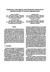
5.2 Performance of base classifiers In Figures 1 and 2, we present the accuracy, the (T P −F P ) spread and the savings of the individual base classifiers on the Chase and First Union credit card data, respectively. The x-axis corresponds to the month of data used to train the base classifiers, starting in October 1995 and ending in September 1996 (the one year span is repeated for the five learning algorithms). Each vertical bar represents a specific base classifier, e.g. the first bar of the left plot of Figure 1 represents the accuracy (83%) of the Bayesian base classifier that was trained on the December 1995 data. The maximum achievable savings a perfect classifier, with respect to the cost model, is $1,470K for the Chase and $1,085K for the First Union data sets. The test set consists of October 1995 - November 1995 data, hence, the performance results of the classifiers corresponding to these months are not included in these plots as these classifiers had been trained on this data. According to the figures, some learning algorithms can be more suitable for one problem (e.g naive Bayes on Chase data) than for another (e.g. naive Bayes on First Union data), even though the two sets are very similar in nature. Overall, it appears that all learning algorithms performed better on the First Union data set than on the Chase data set. On the other hand, note that there are fewer fraudulent transactions in the First Union data and this causes a higher baseline accuracy.
5.3 Pre-Training Pruning Experiments With 50 candidate base classifiers per data site, there are (250 − 50) distinct combinations of base classifiers from which the pruning algorithm has to choose one. In the meta-learning stage, we employed all five learning algorithms to combine the selected base classifiers. The next section, reports the performance results of pruning and meta-learning averaged over al l six data sites. In essence, this experiment is a 6-fold cross validation where each fold is executed in parallel. Results The results from these experiment are displayed in Figures 3, and 4. Figure 3 plots the overall accuracy, the (T P − F P ) spread and the savings (in dollars) for the Chase bank credit card
19
data, and Figure 4 for the First Union data. Each figure contrasts two specialty/coverage based, one diversity-based, a metric-specific pruning method and an additional classifier selection method denoted here as arbitrary. As the name indicates, arbitrary uses no particular strategy to evaluate base classifiers; instead it combines them in a “random” order, i.e. when they become available. The metric-specific pruning methods (which correspond to three different instances of the CCS specialty metric of Section 3.2, namely the accuracy, the (T P −F P ),6 and the cost model) evaluate, rank and select the base-classifiers according to their performance with respect to that metric. For brevity, we plotted only the best performing meta-learning algorithms, the accuracy of the Ripper meta-classifiers and the (T P − F P ) rates and savings of the Bayesian meta-classifiers. The vertical lines in the figures denote the number of base classifiers integrated in the final meta-classifier as determined by the specialty/coverage algorithms. The final Chase meta-classifier for the (T P − F P )/coverage algorithm, for example, combines 33 base classifiers (denoted by the (T P − F P ) vertical line), while the final First Union meta-classifier for the accuracy/coverage algorithm consists of 26 base classifiers (denoted by the accuracy vertical line). In these graphs we have included the intermediate performance results (i.e. the accuracy, (T P − F P ) rates and savings of the partially built meta-classifiers) as well as the performance results of the redundant meta-classifiers would have had, had we used more base-classifiers or not introduced the pruning phase. Vertical lines for the diversity-based and metric-specific pruning algorithms are not shown in these figures as they depend on real-time constraints and available resources as discussed in Section 3.4. The benefits from the pruning methods are clear. Although the algorithms are based on greedy search techniques and heuristically determined termination conditions and there is no guarantee that they will always produce the best ensemble meta-classifier, these experiments demonstrate these algorithms to be successful in computing “good” combinations of base classifiers, at least, with respect, to the three evaluation metrics. Furthermore, these results establish that not all base classifiers are necessary in forming effective meta-classifiers. In all these cases the pruned metaclassifiers are more efficient (fewer base classifiers are retained) and at least as effective (accuracy, (TP-FP), savings) as the complete meta-classifiers and certainly superior to those of the “arbitrary” 6
The CCS/coverage pruning algorithm defined in Section 3.4 iterates through all classes ck , and selects the clas-
sifiers that maximize the CCS(ck ). The fraud detection problem, however, is a binary classification problem, hence the CCS algorithm is, initially, reduced to select the classifiers that maximize CCS(fraud)/coverage, (i.e fT P (fraud) - fF P (fraud)), and furthermore, reduced to (T P − F P ) to match the evaluation metric.
20
pruning method. Using more base-classifiers than selected (denoted by the vertical lines) has no positive impact on the performance of the meta-classifiers. Overall, the pruning methods composed meta-classifiers with 0.7% higher accuracy, 6.2% higher (T P − F P ) spread and $180K/month additional savings over the best single classifier for the Chase data and 1.65% higher accuracy, 10% higher (T P − F P ) spread and $140K/month additional savings over the best single classifier for the First Union data. These pruned meta-classifiers also achieve 60% better throughput, 1% higher (T P − F P ) spread and $100K/month additional savings than the unpruned meta-classifier for the Chase data and 100% better throughput, 2% higher (T P − F P ) spread and $10K/month additional savings for the First Union data. Finally, the meta-classifiers succeeded in improving the performance even over the single classifier trained over the entire data sets (10 months of data for training, 2 months for testing in a 6-fold cross validation fashion). The meta-classifiers increased the accuracy by 0.4%, the (T P −F P ) rate by 4.7% and the savings by $144K/month for the Chase data set and 1.2%, 6.5% and $108K/month for the First Union data set, respectively. Analysis A head to head comparison between the various pruning algorithms seems to point to a contradiction. The simple metric-specific pruning methods choose better combinations of classifiers for the Chase data, while the specialty/coverage-based and diversity-based pruning methods perform better on classifiers for the First Union data. In fact, this observation is more pronounced in most of the plots (not shown here) generated from the meta-classifiers computed by the other learning algorithms. The performance of a meta-classifier, however, is directly related to the properties and characteristics of its constituent base-classifiers. As we have already noted, the more diverse the set of base-classifiers is, the more room for improvement the meta-classifier has. For example, to obtain diverse classifiers from a single learning program Freund and Schapire [12] introduced the boosting algorithm that resamples the data set to artificially generate diverse training subsets. In our experiments, the diversity of the base classifiers is attributed, first, on the use of disparate learning algorithms, and second, on the degree the training sets are different. Although the first factor is the same for both Chase and First Union data sets, we postulate that this is not the case with the second. Recall that the First Union classifiers were trained on subsets of data of equal size and class distribution while the Chase base-classifiers were trained on subsets of data defined according to the date of the credit card transaction, which led to variations in the size of the training sets and the class distributions. As a result, in the Chase bank case, the simple metric-specific pruning
21
algorithm combines the best base-classifiers that are already diverse and hence achieves superior results while the specialty/coverage pruning algorithms combine diverse base-classifiers that are not necessarily the best. On the other hand, in the First Union case, the specialty/coverage pruning algorithms are more effective, since the best base-classifiers are not as diverse. Figures 1 and 2 also support this observation. The performance of the Chase base classifiers varies significantly, even when comparing classifiers computed by the same learning algorithm, indicating higher diversity. Conversely, the First Union classifiers, with the exception of the significantly inferior Bayesian classifiers, lack this diversity especially when comparing classifiers computed by the same learning algorithm. To substantiate this conjecture, 7 we plotted Figure 5 as a means to visualize the diversity among the base classifiers. Each cell in the plot displays the diversity of a pair of base classifiers, with bright cells denoting a high degree of similarity and dark cells high degree of diversity. The bottom right half is allocated to Chase base classifiers while the top left half represents the First Union base classifiers. Each base-classifier is identical to itself as shown by the white diagonal cells. The Bayesian First Union base classifiers, for example, are very similar to each other (light color cells at the bottom right corner of the plot and above the diagonal) and fairly different from the rest (10 dark columns at the left side of the figure), an observation that confirms the results from Figure 2. The diversity plot clearly demonstrates that Chase base classifiers are more diverse than First Union base classifiers. Furthermore, observe that in the First Union data the various pruning algorithms are comparably successful and their performance plots are less distinguishable. A closer inspection on the classifiers composing the pruned sets (C) revealed that the sets of selected classifiers were more “similar” (there were more common members) for First Union than for Chase. Moreover, the inspection showed that for the First Union meta-classifiers, the specialty/coverage based and diversity-based pruning algorithms tended to select mainly the ID3 base-classifiers for being more specialized/diverse8 thus substantiating the conjecture that the primary source of diversity for First Union meta-classifiers is the use of different learning algorithms. If the training sets for First Union were more diverse, there would have been more diversity among the other base-classifiers and presumably more variety in the pruned set. In any event, all pruning methods tend to converge after a certain point. After all, as they add classifiers, their pool of selected classifiers is bound to 7
After all, similarity in performance does not necessarily imply high correlation between classifiers, e.g. it is
possible for two classifiers to have different predictive behavior and exhibit similar accuracy. 8 The ID3 learning algorithm is known to overfit its training sets. In fact, small changes in the learning sets can force ID3 to compute significantly different classifiers.
22
converge to the same set. Note that training classifiers to distinguish fraudulent transactions is not a direct approach to maximizing savings (or the T P − F P spread). In this case, the learning task is ill-defined. The base-classifiers are unaware of the adopted cost model and the actual value (in dollars) of the fraud/legitimate label. The effects of this shortcoming are best demonstrated in Figure 1. The most accurate classifiers are not necessarily the most cost effective. Although the Bayesian base classifiers are less accurate than the Ripper and C4.5 base classifiers, they are by far the best under the cost model. Similarly, the meta-classifiers are trained to maximize the overall accuracy not by examining the savings in dollars but by relying on the predictions of the base-classifiers. In fact, Figure 1 reveals that with only a few exceptions, the Chase base-classifiers are inclined towards catching “cheap” fraudulent transactions and for this they exhibit low savings scores. Naturally, the meta-classifiers are trained to trust the wrong base-classifiers for the wrong reasons, i.e. they trust the base-classifiers that are most accurate instead of the classifiers that accrue highest savings. The superior performance of the simple cost-specific pruning method confirms this hypothesis. The cost-specific pruning method evaluates the base classifiers with respect to the cost model. The algorithm forms meta-classifiers by selecting base-classifiers based on cost savings performance. The performance of this algorithm is displayed in the right plot of Figure 3 under the name “cost”. While the ensemble consists of base classifiers with good cost model performance the meta-classifier exhibits substantially improved performance as well. The curves for the First Union data set were not as distinct since the majority of the First Union base-classifiers happened to catch the “expensive” fraudulent transactions anyway (see Figure 2), so the pruning algorithms were able to form meta-classifiers with the appropriate base classifiers. The same, but to a lesser degree, holds for the (T P −F P ) spread. In general, unless the learning algorithm’s target function is aligned with the evaluation metric, the resulting base- and meta-classifiers will not be able to solve the classification problem as best as possible except perhaps by chance. In such cases, it is often preferable to discard from the ensemble the base classifiers that do not exhibit the desired property. One way to deal with this situation in to use cost-sensitive algorithms, i.e. algorithms that employ cost models to guide the learning strategy. On the other hand, this approach has the disadvantage of requiring significant change to generic algorithms. An alternative, but (probably) less effective technique is to tune the learning problem according to the adopted cost model. In the credit card fraud domain, for example, we can transform the binary classification problem into a 23
multi-class problem by multiplexing the binary class and the continuous amt attribute (properly quantized into several “bins”). The classifiers derived from the modified problem would perhaps fit better to the specification of the cost model and ultimately achieve better results.
5.4 Post-Training Pruning experiments As with the pre-training pruning experiments, the post-training pruning algorithms are evaluated on their ability to choose the best set of base classifiers among the 50 that are available per data site. As before, the final meta-classifiers correspond to the higher level models derived by the same five learning algorithms. The difference in these tests is that the post-training pruning algorithms start with pre-computed (complete or pruned) meta-classifiers and search for less expensive but effective combinations of base classifiers. The experiments examine the effectiveness of the costcomplexity pruning algorithm and compare it against the correlation-based back pruning method. The performance results of the pruned meta-classifiers for the Chase and First Union data sets are presented in Figures 6 and 7, respectively. As with the previous experiments, we display the accuracy (left plots), the (T P − F P ) spreads (middle plots) and the savings (right plots) achieved. According to these figures, in most of the cases, the cost-complexity post-training pruning algorithm computes superior meta-classifiers compared to the correlation-based pruning method. In general, the cost-complexity algorithm is successful in pruning the majority of the base-classifiers without any performance penalties. In contrast, the correlation-based pruned meta-classifiers perform better only with respect to the cost model and only for the Chase data set. This can be attributed to the manner in which the specific meta-classifiers correlate to their base-classifiers and not to the search heuristics of the method. The pruning method favors (retains) the base classifiers that are more correlated to the Bayesian meta-classifier which in this case happens to be the Bayesian base classifiers with the higher cost savings. As a result, the pruned meta-classifiers demonstrate increased savings even compared to the complete meta-classifier. Conversely, the cost-complexity pruning algorithm generates pruned meta-classifiers that best match the behavior and performance of the complete meta-classifiers. Overall, the correlation-based pruning cannot be considered a reliable pruning method unless only a few base classifiers need to be removed, while the cost-complexity algorithm is more robust and appropriate when many base classifiers need to be discarded. The degree of pruning of a meta-classifier within a data site is dictated by the throughput re-
24
quirements of the particular problem. There is trade-off between the throughput and the predictive performance of classification systems. Higher throughput requirements necessitate higher pruning and that implies that only the most important available models can be combined. Fortunately, the cost-complexity pruning algorithm is fairly intelligent in discerning the set of classifiers that is most “important”. Figure 8 demonstrates the algorithm’s effectiveness on the Chase (left) and First Union (right) classifiers by displaying the predictive performance and throughput of the pruned meta-classifiers as a function of the degree of pruning. To normalize the different evaluation metrics and better quantify the effects of pruning, we measured the ratio of the performance improvement of the pruned meta-classifier over the performance improvement of the complete (original) meta-classifiers. In other words, we measured the performance gain ratio G =
PP RU NED −PBASE , PCOMP LET E −PBASE
where PP RU N ED , PCOM P LET E and PBASE denote the performance (accuracy, (T P − F P ) spread and savings) of the pruned meta-classifier, the complete meta-classifier and the best base classifier, respectively. Values of G ≃ 1 indicate pruned meta-classifiers that sustain the performance levels to that of the complete meta-classifier while values of G < 1 indicate performance losses. When only the best base classifier is used, there is no performance improvement and G = 0. In this figure, the black colored bars represent the accuracy gain ratios, the dark gray colored bars represent the (T P − F P ) gain ratios and the light gray bars represent the savings gain ratios of the pruned meta-classifier. The very light gray bars correspond to the relative throughput of the pruned meta-classifier TP to the throughput of the complete meta-classifier TC . To estimate the throughput of the meta-classifiers, we measured the time needed for a meta-classifier to generate a prediction. This time includes the time required to obtain the predictions of the constituents base classifiers sequentially on an unseen credit card transaction, the time required to assemble these predictions into a single meta-level “prediction” vector and the time required for the meta-classifier to examine the vector and generate the final prediction. The measurements were performed on a Personal Computer with a 200MHz Pentium processor running Solaris 2.5.1. These measurements show that cost-complexity pruning is successful in finding Chase meta-classifiers that retain their performance levels to 100% of the original even with as much as 60% of the base classifiers pruned or within 60% of the original with 90% pruning. At the same time, the pruned classifiers exhibit 230% and 638% higher throughput. For the First Union base classifiers, the results are even better. With 80% pruning, the pruned meta-classifiers have gain ratios G ≃ 1 and with 90% pruning they are within 80% of the original performance. The throughput improvement in this case is 5.08 and 9.92 times better, respectively. 25
5.5 Combining Pre-Training and Post-Training Pruning Pre-training pruning and post-training pruning are complementary methods that employ different metrics to discard base classifiers. It is possible to visualize and contrast the manner the different pruning methods select or discard the base classifiers by computing the meta-classifier correlation matrices and by mapping them onto a modified density plot. Figure 9, for instance, displays three plots for the Chase data set that represent the correlation between the meta-classifiers and the base classifiers as selected by the specialty/coverage (left), the correlation-based (middle) and the cost-complexity (right) pruning algorithms, respectively. In these plots, each column corresponds to a single base classifier and each row corresponds to one meta-classifier, with the complete (unpruned) meta-classifier mapped on the bottom row, and the single base classifier mapped to the top. Dark gray cells represent meta-classifiers and base-classifiers that are highly correlated, while white cells identify the pruned base classifiers. The 3-column density plots accompanying the correlation-density plot represent the performance of the individual meta-classifiers, namely their accuracy (left column), their (T P − F P ) spread (middle column) and their savings (right column), with dark colors signifying “better” meta-classifiers. Apart from exposing the relationships between meta classifiers and base classifiers, these plots provide information regarding the order the various base classifiers were selected or discarded. They can be read top-down for the pre-training pruning algorithms and bottom-up for post-training pruning. The specialty/coverage method, for example, begins by selecting a Ripper classifier (which corresponds to the January’96 data) and continues by adding mostly ID3 and CART classifiers. The pruning algorithms examined in this paper can be briefly described as iterative search methods that greedily (without back-tracking) add (in pre-training) or remove (in post-training) one classifier per iteration. Assuming that the data sets and the base classifiers are common to all pruning algorithms, the meta-classifiers enumerated by these methods (recall that the pruning methods discussed do not require intermediate meta-classifiers), depends on the starting point (e.g the first base-classifier selected, the initial meta-classifier, etc.) on the search heuristic (metrics) evaluating the classifiers at each step, and on the portion of the validation data used for the evaluation. As a result, different pruning algorithms compute different combinations of classifiers and search distinct parts of the space of possible meta-classifiers. The correlation plots introduced above can serve as tools for studying the properties and limitations of the various pruning algorithms. Figure 9, for example, demonstrates that the three pruning algorithms consider very 26
different combinations of base-classifiers. The first (Specialty/Coverage) tends to select diverse classifiers (c.f. to Figure 5), the second (correlation-based) clusters the classifiers by the algorithm type, while the third (cost-complexity) forms more complex relationships and thus appears more balanced and robust. By allowing pre-training pruning to compute both the intermediate and the larger meta-classifiers, (in a manner similar to that of Figures 3 and 4), and by applying post-training pruning to the best meta-classifier, it is possible to combine two different parts of the meta-classifier space and produce a final pruned meta-classifier that is even more effective and more efficient. The rationale parallels the strategy used in decision tree algorithms: first grow a large tree to avoid stopping too soon and then prune the tree back to compute subtrees with lower misclassification rate. In this case, post-training pruning is applied to the best intermediate meta-classifier which may not necessarily be the largest (complete) meta-classifier. This is particularly the case when the learning algorithm’s target function is not aligned with the evaluation metric and only a small number of classifiers might be appropriate. Table 2 for the Chase data and Table 3 for the First Union data compare the effectiveness and efficiency of the complete meta-classifiers (first rows) to the most effective meta-classifiers computed by the pre-training pruning algorithms (second rows), the most effective meta-classifiers computed by the combination of the pre-training and the cost-complexity post-training pruning algorithms (third rows) and the most effective meta-classifiers computer by the pre-training and the correlation-based post training pruning algorithms (last rows). Effectiveness is measured by the meta-classifier’s accuracy (first columns) the meta-classifier’s (T P −F P ) spread (second columns) and the meta-classifier’s savings (third columns) each accompanied by its degree of pruning (compared to the complete meta-classifier) and efficiency (relative throughput, denoted as TP /TC ). As expected, there is no single best meta-classifier; depending on the evaluation criteria and the target learning task, different meta-classifiers should be constructed and deployed. According to these experiments, pre-training pruning is able to compute more effective and more efficient meta-classifiers than those obtained by combining all available base classifiers, and post-training pruning and in particular the cost-complexity algorithm is successful in further reducing the size of these meta-classifiers. In fact, the larger the pre-trained pruned meta-classifier is, the larger the degree of additional pruning the cost-complexity algorithm exhibits. The post-training pruning algorithm that is based on the correlation metric, however, provides either limited or, is some cases, no further improvement, e.g. see the (T P − F P ) column of Table 3. Another obser27
vation to note, is that the throughput of a meta-classifier is also a function of its constituent base classifiers. Some classifiers are faster in producing predictions than others (due to size, different representations, implementation details, etc) and this may have a significant effect on the speed of the entire meta-classifier. As an example, observe the two post-trained pruned First Union metaclassifiers with the best (T P − F P ) spreads. They both have the same size, yet they are composed of different base classifiers and for that they exhibit different throughputs.
6 Conclusion In this paper we studied efficient and effective methods that combine multiple models computed over distributed databases into scalable and efficient meta-classifiers. We addressed scalability and efficiency, first, by employing distributed and asynchronous protocols at the architectural level for managing the learning agents across the data sites of the JAM system, and second by introducing pruning algorithms at the data site level to evaluate, retain and use only the most essential classifiers in an ensemble meta-classifier. We introduced several evaluation metrics and pre-training pruning algorithms for selecting classifiers before they are combined into a meta-classifier, and a posttraining pruning algorithm based on the cost-complexity pruning of decision tree for discarding classifiers after being combined into a meta-classifier. On real credit card transaction data sets from two separate institutions we demonstrated that pruning base classifiers in meta-learning can achieve similar or better performance results than the brute-force assembled meta-classifiers but at a substantially reduced computational cost and higher throughput. With the help of correlation-based visualization tools we analyzed base classifiers and meta-classifiers and we established that the suitability of a pre-training pruning method depends on the particular set of candidate base classifiers and the target learning task. Furthermore, we determined cost-complexity post-training pruning methods to be an efficient, intuitive and robust method for discarding the base classifiers and we illustrated that combining cost-complexity pruning and pre-training pruning can yield meta-classifiers with further improved effectiveness and efficiency. In these experiments, we considered only simple one-level meta-classifiers, i.e. meta-classifiers integrating only base classifiers. Our future plans include the extension of these methods to metaclassifier hierarchies. As more databases become available, we expect that the pruning of larger meta-classifier hierarchies will be of even greater importance. 28
We address these two issues by employing meta-learning as a distributed learning method. Then we introduce distributed management protocols among the data sites that provide for the exchange of classifiers among remote sites. We then describe fast methods to evaluate these classifiers, filtering out (pruning) redundant models and deploying only the most essential classifiers to prevent the formation of complex, large and inefficient meta-classifiers.
29
A Appendix Table 1: The Diversity-based (left) and Coverage/Specialty-based (right) pruning algorithms Let C := ∅, N := maximum number of classifiers For i := 1, 2, . . . , |H| - 1 do For j := i, i+1, . . . , |H| do Let dij := the ratio of the instances the Ci and Cj give different predictions Let C ′ := the classifier with the highest accuracy C := C ∪ C ′ , H := H − C ′ For i := 1, 2, . . . , N do For j := 1, 2, . . . , |H| do P|C| Let Dj := 2 · ( k=1 djk )/|C| · (|C| + 1) Let C ′ := the classifier from H with the highest Dj C := C ∪ C ′ , H := H − C ′
Accuracy of Chase base classifiers on Oct.95 - Nov.95 test data
TP - FP spread of Chase base classifiers on Oct.95 - Nov.95 test data
0.89
0.45
900000 Bayes C4.5 CART ID3 Ripper
Bayes C4.5 CART ID3 Ripper
800000 700000
0.4
0.86
TP - FP rate
Total Accuracy
0.87
Savings of Chase base classifiers on Oct.95 - Nov.95 test data
0.5 Bayes C4.5 CART ID3 Ripper
0.85 0.84
Savings in dollars
0.88
Let C := ∅ For all target classes ck , k = 1, 2, . . . , c, do Let E := V Let C k := ∅, Hk := ∅ Until no other examples in E can be covered or Hk = ∅ Let C ′ := the classifier with the best class specialty on target class ck for E C k := C k ∪ C ′ , Hk := Hk − C ′ E := E - examples covered by C ′ C := C ∪ C k
0.35 0.3
600000 500000 400000 300000
0.25
0.83
200000 0.2
0.82 0.81 Sep Feb Jul Dec May Oct Mar Aug Jan Jun Nov Apr Sep Base Classifiers
100000
0.15 Sep Feb Jul Dec May Oct Mar Aug Jan Jun Nov Apr Sep Base Classifiers
0 Sep Feb Jul Dec May Oct Mar Aug Jan Jun Nov Apr Sep Base Classifiers
Figure 1: Base Classifiers: Total accuracy (left), (TP-FP) spread (middle) and savings (right) on Chase credit card data. TP - FP spread of First Union base classifiers on Oct.95 - Nov.95 test data Bayes C4.5 0.7 CART ID3 Ripper 0.65
0.93 0.92
0.91
0.9
0.89 Sep Feb Jul Dec May Oct Mar Aug Jan Jun Nov Apr Sep Base Classifiers
0.6 0.55 0.5 0.45 0.4 0.35 Sep Feb Jul Dec May Oct Mar Aug Jan Jun Nov Apr Sep Base Classifiers
Savings of First Union base classifiers on Oct.95 - Nov.95 test data 800000 Bayes C4.5 CART ID3 700000 Ripper 750000
Savings in dollars
0.75
Bayes C4.5 0.95 CART ID3 Ripper 0.94 TP - FP rate
Total Accuracy
Accuracy of First Union base classifiers on Oct.95 - Nov95 test data 0.96
650000 600000 550000 500000 450000 400000 350000 Sep Feb Jul Dec May Oct Mar Aug Jan Jun Nov Apr Sep Base Classifiers
Figure 2: Base Classifiers: Total accuracy (left), (TP-FP) spread (middle) and savings (right) on First Union credit card data.
Accuracy of Ripper Chase meta-classifiers with Chase base classifiers
TP - FP of Bayes Chase meta-classifiers with Chase base classifiers
0.9
Savings of Bayes Chase meta-classifiers with Chase base classifiers
0.64
950000
0.62
900000
0.6
850000
0.58
800000
0.56 TP - FP rate
Total Accuracy
0.88
savings in dollars
0.89
0.87 Accuracy PCS Coverage Coverage
0.86
0.85
TP-FP PCS Coverage Coverage
0.52 0.5
Arbitrary Accuracy Diversity Accuracy/Coverage PCS/Coverage
0.84
0.54
0.48
Arbitrary TP-FP Diversity TP-FP/Coverage PCS/Coverage
0.46 0.44
0.83 10 15 20 25 30 35 40 number of base-classifiers in a meta-classifier
45
PCS Coverage
700000
Cost Coverage
650000 600000 550000
Arbitrary Cost Diversity Cost/Coverage PCS/Coverage
500000 450000
0.42 5
750000
400000
50
5
10 15 20 25 30 35 40 number of base-classifiers in a meta-classifier
45
50
5
10 15 20 25 30 35 40 number of base-classifiers in a meta-classifier
45
50
Figure 3: Pruning algorithms: Total accuracy (left), (TP-FP) spread (middle) and savings (right) on CHASE credit card data. Accuracy for Ripper First Union meta-classifiers with First Union base classifiers 0.97
TP - FP for Bayes First Union meta-classifiers with First Union base classifiers 0.85
Savings of Bayes Fist Union meta-classifiers with Fist Union base classifiers 950000
0.965
900000
0.8 0.96
PCS Coverage
0.945
Accuracy Coverage
0.94 0.935
Arbitrary Accuracy Diversity Accuracy/Coverage PCS/Coverage
0.93 0.925
0.7 PCS TP-FP Coverage Coverage
0.65
0.6
Random TP-FP Diversity TP-FP/Coverage PCS/Coverage
0.55
0.92
savings in dollars
0.95
TP - FP rate
Total Accuracy
850000
0.75
0.955
10 15 20 25 30 35 40 number of base-classifiers in a meta-classifier
45
50
PCS Coverage
750000
Cost Coverage
700000 Random Cost Diversity Cost/Coverage PCs/Coverage
650000 600000
0.5 5
800000
550000 5
10 15 20 25 30 35 40 number of base-classifiers in a meta-classifier
45
50
5
10 15 20 25 30 35 40 number of base-classifiers in a meta-classifier
45
Figure 4: Pruning algorithms: Total accuracy (left), (TP-FP) spread (middle) and savings (right) on First Union credit card data.
50
Figure 5: Base classifier diversity plot between all pairs of Chase base classifiers (bottom right half) and all pairs of First Union base classifiers (top left half).
Accuracy of Ripper Chase meta-classifiers with Chase base classifiers
TP - FP of Bayes Chase meta-classifiers with Chase base classifiers
0.9
Savings of Bayes Chase meta-classifiers with Chase base classifiers
0.65
900000
850000 0.6
0.89
savings in dollars
800000 TP - FP rate
Total Accuracy
0.895
0.55
0.5
750000 700000
650000
0.885 0.45
Cost Complexity Correlation 0.88
Cost Complexity Correlation
0.4 5
10 15 20 25 30 35 40 number of base-classifiers in a meta-classifier
45
50
Cost Complexity Correlation
600000
550000 5
10 15 20 25 30 35 40 number of base-classifiers in a meta-classifier
45
50
5
10 15 20 25 30 35 40 number of base-classifiers in a meta-classifier
45
50
Figure 6: Post-Pruning algorithms on Chase data: Total accuracy (left), (TP-FP) spread (middle) and savings (right). Accuracy for Ripper First Union meta-classifiers with First Union base classifiers 0.968
TP - FP for Bayes First Union meta-classifiers with First Union base classifiers 0.84
Savings of Bayes Fist Union meta-classifiers with Fist Union base classifiers 960000
0.82
940000
0.966 0.964
0.958 0.956 0.954
savings in dollars
0.96
TP - FP rate
Total Accuracy
920000
0.8
0.962
0.78 0.76
0.74
0.952
Cost Complexity Correlation
0.95
10 15 20 25 30 35 40 number of base-classifiers in a meta-classifier
45
50
860000
Cost Complexity Simple
820000
0.7 5
880000
840000 Cost Complexity Correlation
0.72
0.948
900000
800000 5
10 15 20 25 30 35 40 number of base-classifiers in a meta-classifier
45
50
5
10 15 20 25 30 35 40 number of base-classifiers in a meta-classifier
45
Figure 7: Post-Pruning algorithms on First Union: Total accuracy (left), (TP-FP) spread (middle) and savings (right).
50
Figure 8: Bar charts of the accuracy (black bars), TP - FP (dark gray bars), savings (light gray bars) and throughput (very light gray bars) of the Chase (right) and First Union (left) meta-classifiers as a function of the degree of pruning.
Figure 9: Selection of classifiers on Chase data: Specialty/Coverage Pruning (left) Correlation Pruning (middle) and Cost-Complexity Pruning (right). Table 2: Performance and Relative Throughput of the Best Chase Meta-Classifiers Complete Pre Training + Post (CC) + Post (LC)
Accuracy 89.57 89.66 89.66 89.62
Pruning 0% 30 % 72 % 38 %
TP /TC 1.0 1.43 3.18 1.6
TP - FP 62.05 63.13 63.1 63.13
Pruning 0% 54 % 64 % 54 %
TP /TC 1.0 2.01 2.57 2.01
Savings 818K 935K 923K 931K
Pruning 0% 90 % 92 % 94 %
TP /TC 1.0 6.5 8.25 10.11
Table 3: Performance and Relative Throughput of the Best First Union Meta-Classifiers Complete Pre Training + Post (CC) + Post (LC)
Accuracy 96.47 96.53 95.53 96.53
Pruning 0% 54 % 72 % 54 %
TP /TC 1.0 2.48 3.87 2.48
TP - FP 82.53 84.61 84.52 84.69
Pruning 0% 72 % 78 % 78 %
TP /TC 1.0 4.33 4.78 5.25
Savings 935K 940K 940K 940K
Pruning 0% 8% 48% 12%
TP /TC 1.0 1.16 2.32 1.25
References [1] K. Ali and M. Pazzani. Error reduction through learning multiple descriptions. Machine Learning, 24:173–202, 1996. [2] L. Breiman. Heuristics of instability in model selection. Technical report, Department of Statistics, University of California at Berkeley, 1994. [3] L. Breiman. Stacked regressions. Machine Learning, 24:41–48, 1996. [4] L. Breiman, J. H. Friedman, R. A. Olshen, and C. J. Stone. Classification and Regression Trees. Wadsworth, Belmont, CA, 1984. [5] C. Brodley and T. Lane. Creating and exploiting coverage and diversity. In Work. Notes AAAI-96 Workshop Integrating Multiple Learned Models, pages 8–14, 1996. [6] C.Brodley. Addressing the selective superiority problem: Automatic algorithm/model class selection. In Proc. 10th Intl. Conf. Machine Learning, pages 17–24. Morgan Kaufmann, 1993. [7] P. Chan. An Extensible Meta-Learning Approach for Scalable and Accurate Inductive Learning. PhD thesis, Department of Computer Science, Columbia University, New York, NY, 1996. [8] P. Chan and S. Stolfo. Meta-learning for multistrategy and parallel learning. In Proc. Second Intl. Work. Multistrategy Learning, pages 150–165, 1993. [9] W. Cohen. Fast effective rule induction. In Proc. 12th Intl. Conf. Machine Learning, pages 115–123, 1995. [10] T.G. Dietterich. Machine learning research: Four current directions. AI Magazine, 18(4):97– 136, 1997. [11] Y. Freund and R. Schapire. A decision-theoretic generalization of on-line learning and an application to boosting. In Proceedings of the Second European Conference on Computational Learning Theory, pages 23–37. Springer-Verlag, 1995. [12] Y. Freund and R. Schapire. Experiments with a new boosting algorithm. In Proc. Thirteenth Conf. Machine Learning, pages 148–156, 1996.
[13] Michael J. Greenacre. Theory and Application of Correspondence Analysis. Academic Press, London, 1984. [14] L. Hansen and P. Salamon. Neural network ensembles. IEEE Trans. Pattern Analysis and Mach. Itell., 12:993–1001, 1990. [15] R.A. Jacobs, M.I. Jordan, S. J. Nowlan, and G. E. Hinton. Adaptive mixture of local experts. Neural Computation, 3(1):79–87, 1991. [16] Michael I Jordan and Robert A. Jacobs. Hierarchical mixtures of experts and the em algorithm. Neural Computation, 6:181–214, 1994. [17] A. Krogh and J. Vedelsby. Neural network ensembles, cross validation, and active learning. In G. Tesauro, D. Touretzky, and T. Leen, editors, Advances in Neural Info. Proc. Sys. 7, pages 231–238. MIT Press, 1995. [18] S. Kwok and C. Carter. Multiple decision trees. In Uncertainty in Aritificial Intelligence 4, pages 327–335, 1990. [19] M. LeBlanc and R. Tibshirani. Combining estimates in regression and classification. Technical Report 9318, Department of Statistics, University of Toronto, Toronto, ON, 1993. [20] D. Margineantu and T. Dietterich. Pruning adaptive boosting. In Proc. Fourteenth Intl. Conf. Machine Learning, pages 211–218, 1997. [21] C. Merz. Using correspondence analysis to combine classifiers. Machine Learning, 1998. to appear. [22] C. Merz and M. Pazzani. A principal components approach to combining regression estimates. Machine Learning, 1998. to appear. [23] R. Michalski. A theory and methodology of inductive learning. In R. Michalski, J. Carbonell, and T. Mitchell, editors, Machine Learning: An Artificial Intelligence Approach, pages 83– 134. Morgan Kaufmann, 1983. [24] M. Minksy and S. Papert. Perceptrons: An Introduction to Computation Geometry. MIT Press, Cambridge, MA, 1969. (Expanded edition, 1988). [25] T. Mitchell. Generalization as search. Artificial Intelligence, 18:203–226, 1982.
[26] David W. Opitz and J. Jude W. Shavlik. Generating accurate and diverse members of a neural-network ensemble. Advances in Neural Information Processing Systems, 8:535–541, 1996. [27] M. P. Perrone and L. N. Cooper. When networks disagree: Ensemble methods for hydrid neural networks. Artificial Neural Networks for Speech and Vision, pages 126–142, 1993. [28] A. Prodromidis and S. Stolfo. Mining databases with different schemas: Integrating incompatible classifiers. In Proc. 4rd Intl. Conf. Knowledge Discovery and Data Mining, 1998. [29] A. L. Prodromidis. On the management of distributed learning agents. Technical Report CUCS-032-97 (PhD Thesis proposal), Department of Computer Science, Columbia University, New York, NY, 1997. [30] F. Provost and T. Fawcett. Analysis and visualization of classifier performance: Comparison under imprecise class and cost distributions. In Proc. Third Intl. Conf. Knowledge Discovery and Data Mining, pages 43–48, 1997. [31] F. Provost and T. Fawcett. Robust classification systems for imprecise environments. In Proc. AAAI-98. AAAI Press, 1998. [32] F. Provost and V. Kolluri. Scaling up inductive algorithms: An overview. In Proc. Third Intl. Conf. Knowledge Discovery and Data Mining, pages 239–242, 1997. [33] J. R. Quinlan. Induction of decision trees. Machine Learning, 1:81–106, 1986. [34] J. R. Quinlan. C4.5: programs for machine learning. Morgan Kaufmann, San Mateo, CA, 1993. [35] R. Schapire. The strength of weak learnability. Machine Learning, 5:197–226, 1990. [36] S. Stolfo, W. Fan, W. Lee, A. Prodromidis, and P. Chan. Credit card fraud detection using meta-learning: Issues and initial results. Working notes of AAAI Workshop on AI Approaches to Fraud Detection and Risk Management, 1997. [37] S. Stolfo, W.D. Fan, A. Prodromidis W.Lee, S. Tselepis, and P. K. Chan. Agent-based fraud and intrusion detection in financial information systems. Submitted to IEEE Symposium on Security and Privacy, 1998.
[38] S. Stolfo, A. Prodromidis, S. Tselepis, W. Lee, W. Fan, and P. Chan. JAM: Java agents for meta-learning over distributed databases. In Proc. 3rd Intl. Conf. Knowledge Discovery and Data Mining, pages 74–81, 1997. [39] Volker Tresp and Michiaki Taniguchi. Combining estimators using non-constant weighting functions. Advances in Neural Information Processing Systems, 7:419–426, 1995. [40] D. Wolpert. Stacked generalization. Neural Networks, 5:241–259, 1992.