Abstract. Cube Pruning is a fast method to explore the search space of a beam decoder. In this paper we present two modifi- cations of the algorithm that aim to ...
Faster Cube Pruning Andrea Gesmundo, James Henderson Department of Computer Science University of Geneva {andrea.gesmundo, james.henderson}@unige.ch
Abstract Cube Pruning is a fast method to explore the search space of a beam decoder. In this paper we present two modifications of the algorithm that aim to improve the speed and reduce the amount of memory needed at execution time. We show that, in applications where Cube Pruning is applied to a monotonic search space, the proposed algorithms retrieve the same K-best set with lower complexity. When tested on an application where the search space is approximately monotonic (Machine Translation with Language Model features), we show that the proposed algorithms obtain reductions in execution time with no change in performance.
1. Introduction Since its first appearance in [2], Cube Pruning (CP) gained popularity in the Machine Translation community. Hierarchical or Tree-based Machine Translation models rely on Cube Pruning for decoding. Current research in such Tree-based models builds translation systems that more closely model the underlying recursive structure of languages, and produce more syntactically meaningful translations than Phrase-Based models. On the other hand, the nonsyntactically motivated Phrase-Based Models have linear decoding time, because in practice they use a reordering limit. For Tree-based models, decoding is not linear with respect to sentence length. This higher complexity of Tree-based model decoding leads to a higher execution time. For this reason, real time systems that involve an automatic translation step (such as spoken dialogue systems, or real time text translation systems) often prefer Phrase Based models. With this work we investigate how to improve the speed of Tree-based models by reducing the Cube Pruning decoding complexity without affecting the accuracy of the decoding. In [2], Cube Pruning is presented as an adaptation of the Lazy Algorithm [6] to the Hiero Model [1]. The name “Cube” Pruning comes from the fact that Hiero Model uses a binarised Synchronous Context Free Grammar; therefore at each node of the decoding hypergraph any combination of a rule with the two possible children must be considered, resulting in a three dimensional search space. But the use of Cube Pruning is not necessarily limited to the Machine Translation field or to a three dimensional search space. Lately CP is referred to as a general method for fast and
inexact beam decoding that can be applied whenever certain conditions occur. [5] shows that CP can be viewed as a specialisation of A* for a specific search space with specific heuristics. CP’s generality allows its application to other tasks such as Parsing [6] and Word Alignment [8]. Any task using CP can take advantage of the improvements described in this paper, either in monotonic search spaces or in cases where there are perturbation factors that could create areas of non-monotonicity in the search space. This second case of an approximately monotonic search space occurs in many real word applications, such as the case of Machine Translation decoding with Language Model features, as clearly explained in Section 5 of [2]. We begin by describing the monotonic search space case in Section 2, first stating the problem formally, then reviewing the Lazy Algorithm and introducing the two algorithms we propose as improvement. Section 3 describes the approximately monotonic search space case. It explains how Cube Pruning handles the perturbations of the search space and then shows how the two proposed algorithms can be extended as well. Section 4 reports experiments to test the proposed algorithm and to compare them with Cube Pruning. Finally, Section 5 further investigates the differences in behaviour between Cube Pruning and the proposed algorithms.
2. Monotonic Search Space Cube Pruning is a solution to the problem of finding the best k results of the product of n elements selected from each of n ordered lists. All the applications of Cube Pruning can be reduced to this simple problem. Formally we can state the problem as follows: Problem 1. As input we have: • A set L, containing N = |L| ordered lists Ln | 1 ≤ n ≤ N . We refer to the i-th element of the list Ln as xn,i ∈ X . • An ordering function min≤ , that allows us to compare elements of X , and sort the lists in L. • An operator ⊙ with monotonic property, so that if x′ , x′′ , x ˆ ∈ X and x′ min≤ x′′ then (x′ ⊙ˆ x)min≤ (x′′ ⊙ xˆ)
• The size of the output beam k. As solution of the problem we want: • The ordered list “best-k” containing the top k elements of P. Where P is the set of the results obtained from the ⊙-product of n elements selected from each of the n ordered lists in L: K P≡{ xn,in | xn,in ∈ Ln , 1 ≤ in ≤ |Ln |} 1≤n≤N
(1) Formally: best-k ≡ {xi |1 ≤ i ≤ k, xi ∈ P, ∀ˆ x ∈ (P−best-k), x ˆmin≤ xi } (2) Following [4], it is possible to interpret ⊙ and min≤ respectively as ⊗ and ⊕ (the two binary operations of a semiring) and show the relation between the stated problem and the general definition of bottom-up parsing. We show the correspondence between Problem 1 and common problems where Cube Pruning is applied. As an example, consider a Probabilistic Context Free Grammar (PCFG) Parser. Problem 1 is the one that must be solved during bottom up decoding at each node of the hypergraph. The PCFG decoder has to choose the best k derivations that lead to the generation of the span [i, j] associated with the node. If using only context free features, the score of the derivation is given by summing the log-probability score of the rule R with the scores of the derivations related to the children of R. To show the correspondence between Problem 1 and the parsing example, given a rule R, we make these associations: • xn,i is the score of a derivation for the n-th child of R. • Ln is the ordered list of scores of the derivations correspondent to the n-th child of R. • X is the set of possible values for the scores, for example R, set of the real numbers. • The two binary functions min≤ and ⊙ are respectively ≤ and +. The same correspondence holds for hierarchical Machine Translation decoding, which can be seen as a Synchronous PCFG decoder. Similarly we can find correspondences with other problems whose solution involves the use of Cube Pruning, since they are based on bottom-up parsing techniques, as for example in the case of [8] for Hierarchical Word Alignment. 2.1. Lazy Algorithm We describe here how to solve the stated problem using the Lazy Algorithm presented in [6]. This method is the base for the Cube Pruning algorithm. CP extends the Lazy Algorithm to approximately-monotonic search spaces, as discussed in section 3.
If the lists in L were not sorted, a brute force solution would be to compute all the possible results, sort them and pick the best k. But having defined an ordering function min≤ and a monotonic operator ⊙, it is possible to find the solution without computing all the possible results. To simplify the explanation, we introduce new notation. ˆ= We denote x ˆ = x1,i1 ⊙ x2,i2 ⊙ · · · ⊙ xN,iN with x φ(v), where v is the vector of the indexes of the elements in the lists Ln , v ≡< i1 , i2 , · · · , iN >. We can interpret v as coordinates in a N -dimensional space, that is our search space S, and φ(·) can be seen as a function that maps points in the search space S to values in X : P ≡ {φ(u)|u ∈ S}. We define 1 to be the vector of length N whose elements are all 1, and define bi to be the vector of length N whose elements are all 0 except for bii = 1. The Lazy Algorithm solves Problem 1 proceeding recursively. At each iteration a new element of the best-k list is found. The element φ(1) is added to the best-k list at the first iteration. Because of our assumptions, we know that φ(1) is the best element in S. After adding an element to the best-k list, all the neighbouring elements are visited. Formally the set of neighbouring elements Vv of v is defined as: Vv ≡ {u = v + bi |1 ≤ i ≤ N, u ∈ S}
(3)
Then each neighbour is added to a Queue of Candidates Q if it is not already in it. For all the iterations following the first, the best element of the queue is moved to the best-k and the loop iterate inserting in Q all its neighbours. The algorithm terminates when either the Queue is empty or the best-k list has k elements. So the number of iterations is min(|S|, k). Figure 1 (a) pictures an example for the Lazy Algorithm for a bi-dimensional case N = 2. Algorithm 1 illustrates the Lazy Algorithm. At line 2 the queue Q is initialised inserting the origin element 1. At line 3 the best-k list is initialised as an empty list. The main loop starts at line 4, that will terminate either when the bestk list is full, or when the queue is empty; this second case occurs when the search space contains less than k elements. At line 5, as first step of the loop, the best element in Q is popped and named v. At line 6 v is inserted in the bestk. From line 7 to line 11 the algorithm iterates over all the neighbouring elements of v, and add them to Q. The test at line 8 checks that the element to be inserted in Q is not already into Q. The pseudocode for the function that retrieves the neighbouring elements is listed between line 13 and line 20. This function implements the definition of Vv . At line 14 Vv is initialised as an empty set. The loop between line 15 and line 20 iterates over all the coordinates of v. Each neighbour is created at line 16 adding 1 to v at the current coordinate. The new element is added in Vv at line 18. The test at line 17 is needed to check that the incremented coordinate is still inside the valid range of values, and points to an actual element in Li . To find the best k elements, the Lazy Algorithm avoids computing the φ(·) score for all the elements in the search
Algorithm 1 Lazy Algorithm 1: function MainLoop (L, ⊙, min≤ , k) : best-k 2: Q ← {1}; 3: best-k ←empty list; 4: while |best-k| < k and |Q| > 0 do 5: v ← get-min≤(Q); 6: insert(best-k, v); 7: for all v′ ∈ NeighboursOf(v) do 8: if v′ ∈ / Q then 9: insert(Q, v′ ); 10: end if 11: end for 12: end while 13: 14: 15: 16: 17: 18: 19: 20:
procedure NeighboursOf ( v ): Vv Vv ← empty set; for 1 ≤ i ≤ |v| do v∗ ← v + bi if vi∗ ≤ |Li | then insert(Vv , v∗ ); end if end for
space S. It just needs to compute those best-k along with few other elements that remain in the candidate queue. Note that in the monotonic search space there is no approximation; the algorithm finds the correct best-k set. This will not be true for the approximately monotonic case, as we will see in Section 3. To improve the Lazy Algorithm we cannot avoid computing the best k elements. What can be done is to reduce the number of elements that are in the queue during execution time, and the number of leftover elements that remain in the queue at the end of the execution. A shorter queue needs less memory at run time and consumes less time adding the new elements in sorted order. Furthermore, if the queue at the end of the execution is shorter, we save computation time avoiding computing elements that are not relevant for the output. 2.2. Algorithm 2 Algorithm 2 is the first of the two algorithms we propose as improvement. To introduce it, we focus on a detail of the Lazy Algorithm: before adding a neighbour element in Q, the algorithm needs to check that it has not already been added (see Algorithm 1 line 8). At the implementation level, this check requires either a search in Q (O(log|Q|)) or an additional hash table that allows finding the response in constant time but needs to be maintained as Q changes. This check is needed because an element can be in the set of neighbours of more than one parent element. To define the new algorithm we change the definition of neighbouring elements Vv . For an element v we denote the set of parent elements with
Figure 1: Examples of processing for the three algorithms. As input is given L with N = 2, and L1 ≡ {1, 5, 9, 11}, L2 ≡ {1, 6, 8, 13} sorted lists. For each algorithm are depicted the first 5 iterations. Shaded cells denote elements in the candidate queue, white cells denote elements added in the best-k output list. (a) Lazy Algorithm, (b) Algorithm 2 having vertical dimension with index 1 and horizontal dimension with index 2, (c) Algorithm 3.
Av ≡ {u|v ∈ Vu , u ∈ S}
(4)
We define a new neighbouring elements set Vv′ such that contains a single element. We propose the following definition for Vv′ : A′v
Vv′ ≡ {u = v + bi |∀j < i, vj = 1, 1 ≤ i ≤ N, u ∈ S} (5) Where vj is the j-th coordinate of the vector v =< v1 , v2 , · · · , vN >. As we can see from the definition, Vv′ ⊆ Vv . Vv′ contains the elements of Vv that have all unit values for the coordinates preceding the one updated. For example: v + b1 is always added in Vv′ ; v + b2 is added only if v1 = 1; and in general v + bi is added only if {v1 , v2 , · · · , vi−1 } are all 1. In this setting, it becomes necessary to have an order of the coordinates of v. This means that we need to set an ordering of the elements in L, and L becomes an ordered list rather than a set. This can be seen as deciding an order for the dimensions of the search space S. Having defined Vv′ , we can consider the set of parent elements of v : A′v ≡ {u|v ∈ Vu′ , u ∈ S}. Now we prove that A′v contains only one element for any v 6= 1. Theorem 1. For any element v 6= 1 in the search space S, we have that |A′v | = 1. Proof. By contradiction: • Assume that there is an element v for which | A′v | > 1. • Let u, w ∈ A′v , u 6= w.
• From the definition of A′v , we have that: v ∈ Vu′ and ′ v ∈ Vw • From the definition of V·′ , we have that: v = u + bi , v = w + bj and we have also that ux = 1 ∀ x < i, wy = 1 ∀ y < j, with 1 ≤ i, j ≤ N . • v = u + bi ∧ v = w + bj ⇒ u = w + bj − bi To conclude we distinguish three cases: • if i = j then: u = w + bj − bi = w and this cannot be because it is in contradiction with u 6= w. • if i < j then: From definition of bi we have that: bji = 0 , bii = 1 From i < j and the definition of V ′ we have that: wi = 1 Therefore : ui = wi + bji − bii = 0 But this assignment of values cannot be because no vector v ∈ S can have coordinate with value 0 since the indexing of the lists in L start from 1 by definition. • Similarly if i > j. We showed by contradiction that A′v cannot contain two different elements. Therefore |A′v | ≤ 1. Now consider any v 6= 1, and let i be the index of the first coordinate in the sequence so that vi > 1. We compute u = v − bi , then from the definition of V ′ we have that v ∈ Vu′ . And we can state that for v 6= 1 we have that |A′v | > 0. Combining |A′v | ≤ 1 and |A′v | > 0, it follows that ′ |Av | = 1. Having defined how to retrieve the neighbours, it’s straightforward to write the new algorithm, given as pseudocode in Algorithm 2. Algorithm 2 does not need to check if the neighbours are already in Q. Therefore the test that was done at line 8 of Algorithm 1 is removed. This allows us to avoid the use of a hash table or the execution of a O(log|Q|) search on Q. The new N eighboursOf () procedure is really similar to the first version. Only the test at line18 is added to break the loop when the first coordinate in the sequence that has a value different from 1 is found. The loop break leads to a smaller set of neighbours and therefore a smaller Q and less time spent in the loop. Since most of the elements in the search space have first coordinate with value different from 1, the loop will execute only the first round in most of the cases. Figure 1 (b) illustrates an example for Algorithm 2 for a bidimensional case N = 2, where the vertical dimension has index 1 and the horizontal has index 2. Having defined this new algorithm we need to prove that it solves Problem 1. The proof below shows that the Algorithm 2 outputs the best-k list, that contains the top k elements in S.
Algorithm 2 1: function MainLoop (L, ⊙, min≤ , k) : best-k 2: Q ← {1}; 3: best-k ←empty list; 4: while |best-k| < k and |Q| > 0 do 5: v ← get-min≤(Q); 6: insert(best-k, v); 7: for all v′ ∈ NeighboursOf(v) do 8: insert(Q, v′ ); 9: end for 10: end while 11: 12: 13: 14: 15: 16: 17: 18: 19: 20: 21:
procedure NeighboursOf ( v ): Vv′ Vv′ ← empty set; for 1 ≤ i ≤ |v| do v∗ ← v + bi if vi∗ ≤ |Li | then insert(Vv′ , v∗ ); end if if vi 6= 1 then break; end if end for
Theorem 2. Algorithm 2 solves Problem 1. Proof. By induction on the iterations: • Base case: At the first iteration, 1 is added to best-k. Having monotonic search space and ordered lists, this is the best element in S. • Induction step: At the x-th iteration, the best-k list contains already the top x − 1 elements and a new element v is added from Q. Now we focus on the the set of elements in the search space that are “better” than v, formally: B ≡ {u|φ(u) ≤ φ(v), u ∈ S}. Then we distinguish three cases: – u ∈ B is a candidate in Q: This event cannot occur because in this case u would have been chosen instead of v. – u ∈ B has not been considered (u ∈ / Q, u ∈best/ k) : Now we recursively apply A′ to u and its ancestors, until we find the unique path that connects 1 with u, path: < 1, w1 , · · · , wl , u >. From the monotonicity of search space and definition of A′ we have that: φ(1) ≤ φ(w1 ) ≤ · · · ≤ φ(wl ) ≤ φ(u). Therefore all elements in path are in B. Knowing that 1 is already in best-k and u hasn’t been added in Q, from the definition of Algorithm 2, we know that there is an element in path that
has been added in Q but has not yet been moved into best-k. But this cannot happen since there would be a w ∈ B candidate in Q. – u ∈ B is in best-k: By exclusion this is the only possible case. So we can state that all elements in B are in best-k: B ⊆ best-k. Considering the loop invariant stated above: “at the x-th iteration, best-k list contains already the top x − 1 elements”, we know that best-k cannot contain elements that are “worst” than v, therefore: B ≡ best-k. We conclude that all the elements that are “better” than v are already in best-k, and there are no “better” element outside best-k list. This proves that at the end of the x-th iteration, best-k contains the best x elements. As we explained, for this algorithm we need to specify an order of the coordinates of the search space. It is indifferent in which order we put the coordinates, in the monotonic search space the algorithm will retrieve the same best-k. But the set of elements that are in the queue will be different. For example, if in Figure 1 (b) we wanted to picture the same example but with reversed dimension order (horizontal dimension with index 1, and vertical with index 2), at the second step we would have the element with score 11 in Q, in the fourth step we would not have the element with score 13, and in the last step we would have the element with score 15 instead of the one with score 13. These differences in Q will affect the decoding in the approximately monotonic search space, as will be discussed in Section 3. 2.3. Algorithm 3 Now we introduce the second proposed variation of the Lazy Algorithm. To explain the intuition behind Algorithm 3, consider Figure 1 (a). At the first round we insert 2 in the best-k, then 6 and 7 are added in the queue as candidates. In the second round we pick the smaller element from Q and move it to best-k. Following Lazy Algorithm we need to add all the neighbours of 6 in the queue. Among the neighbours of 6 there is 11. Before adding 11 in Q, we could notice that one of its ancestors, 7, is still in Q. Thus it is certain that at the next round 11 will not be selected to be moved in best-k. So its presence in Q is useless until 7 is selected. Anyway, after 7 is picked, the algorithm will try again to insert 11 in Q. Therefore we can avoid adding 11 at this step and just add 10 as neighbour of 6. In general we can say that it is possible to avoid adding an element to Q until all its ancestors are in the best-k list. Algorithm 3 uses the same Vv and Av as the one defined for the Lazy Algorithm. The difference is in the policy with which Q is updated. The pseudocode for Algorithm 3 is reported below. We can see that the pseudocode for Algorithm 3 is very similar to the pseudocode for the Lazy Algorithm. The only difference
Algorithm 3 1: function MainLoop (L, ⊙, min≤ , k) : best-k 2: Q ← {1}; 3: best-k ←empty list; 4: while |best-k| < k and |Q| > 0 do 5: v ← get-min≤(Q); 6: insert(best-k, v); 7: for all v′ ∈ NeighboursOf(v) do 8: if Av′ ⊆best-k then 9: insert(Q, v′ ); 10: end if 11: end for 12: end while 13: 14: 15: 16: 17: 18: 19: 20:
procedure NeighboursOf ( v ): Vv Vv ← empty set; for 1 ≤ i ≤ |v| do v∗ ← v + bi if vi∗ ≤ |Li | then insert(Vv , v∗ ); end if end for
is at line 8: before adding any of the neighbours of v, we check that all the predecessors of the neighbour are already in the best-k list: Av′ ⊆ best-k. Obviously we no longer need to check if the neighbour v′ is in the queue, because there is no risk that an element is added twice, since every element is added to the queue only in the iteration where the last of its predecessor is added in best-k. As we observed in Algorithm 2: avoiding the statement at line 8 of the Lazy Algorithm allows us to avoid using an additional hash table. Unfortunately, for Algorithm 3 we replace that statement with: Av′ ⊆ best-K, that needs a similar data structure. Furthermore we need to repeat the query a number of times proportional to |Av′ |. Fortunately this number is proportional to the number of dimensions in the search space and that is constant or bounded in most cases. For example in Machine Translation it is preferable to use a grammar composed by binarised rules, in which case |Av′ | ≤ 2. Now we show that Algorithm 3 solves Problem 1. Since the proof is similar to the proof of Theorem 2, we just prove the step that is different. The rest of the proof is done by induction on the iterations exactly following the proof for Theorem 2. Theorem 3. At the x-th iteration of Algorithm 3, the best-k list contains the top x − 1 elements and a new element v is added from Q. Let B ≡ {u|φ(u) ≤ φ(v), u ∈ S}, being the set of elements in S that are “better” than v. Then B ⊆ bestk. Proof. • u ∈ B is candidate in Q: In this case u would have been picked instead of v.
• u ∈ B has not been considered (u ∈ / Q, u ∈ / bestk): Let’s define function γ(·) : S → N, so that PN γ (u) = i=1 ui . From the monotonicity of the search space, we can state that: Au ⊆ B. Therefore Au ∩ Q = ∅. From the definition of the update policy of Q for Algorithm 3, we can say that not all the elements of Au are in best-k, since otherwise u would have already been added in Q. We conclude that there must be an element w1 ∈ Au that has not been considered yet. If we apply the same reasoning recursively, we have that there exists a w2 ∈ Aw1 that has not been considered, and a w3 ∈ Aw2 that has not been considered, and so on. Now we can find where this sequence leads using the γ(·) function: if γ(u) = K then, from how Vw1 is defined, we have that γ(w1 ) = K − 1 and γ(w2 ) = K − 2 and so on. Repeating the iteration K − N times, we reach the element wx such that γ(wx ) = N . Given that N = |L| is the number of dimensions of the search space, the only element wx for which γ(wx ) = N is 1. Now we have reached an absurd because 1 cannot be in the chain of elements that have not been considered. Having shown that every element in B must have already been considered and cannot be in Q, we have to conclude that: all elements in B have been already moved into best-k. Therefore B ⊆ best-k. Compared to Lazy Algorithm, we expect Algorithm 3 to be faster since it uses the minimal number of candidates in the queue. Compared to Algorithm 2, Algorithm 3 also puts fewer elements in Q but needs to use an additional data structure, such as an hash table. Given this analysis, we can’t be sure whether Algorithm 2 or Algorithm 3 is faster, so we will address this issue in the empirical experiments in section 4. We have shown that the three algorithms return the same best-k list in a monotonic search space environment. In the next section we discuss the case of approximately monotonic search spaces, and how we expect the behaviour of the 3 algorithms to change. Later we will compare our expectations with the empirical results.
3. Approximately Monotonic Search Space This section describes the approximately monotonic search space case, shows the correspondence with some popular applications, and describes how the algorithms introduced for the monotonic case can be extended. In the approximately monotonic search space we still have the set of ordered lists L, the ordering function min≤ , and the monotonic operator ⊙ as we defined them in Section 2. The main difference is that instead of computing the ⊙-product of the single input items: x ˆ = x1,i1 ⊙ x2,i2 ⊙ · · · ⊙ xN,iN , in the approximately monotonic case we have to add a perturbation element: xˆ = x1,i1 ⊙ · · · ⊙ xN,iN ⊙ ∆(i1 , · · · , iN )
(6)
Where ∆(i1 , · · · , iN ) is the perturbation function, ∆(·) : S → X . For brevity we define ψ(v) = φ(v) ⊙ ∆(v). The perturbation function ∆(·) must have two properties: • ∆(·) is not proportional to φ(·), formally: ∃ v, u ∈ S, φ(v) ≤ φ(u) such that ∆(v) � ∆(u). Therefore we could have cases where φ(v) ≤ φ(u), but ψ(v) � ψ(u). In those cases the search space described by ψ(·) has some perturbations and it could have areas of non-monotonicity. • The magnitude of ∆(v) must be smaller or proportional to φ(v). In cases where |∆(v)| ≫ |φ(v)| the search space could become fully non-monotonic. In order to successfully apply Cube Pruning and the proposed algorithms, we need to have an approximately monotonic search space. Examples of adding a perturbation function ∆(·) are adding the Language Model in a Machine Translation system, or adding global features in a CKY parser. More generally, a perturbation function ∆(·) can add non-local contextual factors in the scores used to define Problem 1. Given this definition of the approximately monotonic search space in terms of function ψ(·), to guarantee finding the best-k list would require exploring the entire space. This is because the function ∆(·) could be any function with the two stated properties, and any distortion in the search space could be introduced. If we apply the Lazy Algorithm to the approximately monotonic search space, it would compute a small corner of the space, and we would obtain an approx˜ imate best-k list: best-k. As described in [2], Cube Pruning applies the Lazy Algorithm using a margin parameter ǫ to control the level of uncertainty about whether the true best-k has been found. Cube Pruning continues to search the ˜ space until the best-k contains k elements and all the elements v ∈ S such that ψ(v) ≤ ψ(u∗ ) ⊙ ǫ have been com˜ puted, where u∗ is the “worst” element in best-k. Thus the algorithm does not stop as soon as the list is full, but continues to search in the neighbourhood of the top corner of the search space for a while. Applications with a small ratio R = |∆(v)|/|φ(v)| are closer to the monotonic case, and we can use a small ǫ and still have good quality results. When R is big, we need to tune ǫ to a higher value, which will slow down execution because more of the space is searched. In either case, Cube Pruning is not an exact search technique and ˜ will return an approximate best-k list. We can apply the same reasoning that led us from Lazy Algorithm to Cube Pruning to the proposed Algorithm 2 and Algorithm 3, and straightforwardly deduce the approximately monotonic version of the two algorithms. Accordingly, the proposed algorithms use a margin parameter ǫ to control the uncertainty in finding the best-k. As with Cube Pruning, the proposed algorithms output an approxi˜ mate best-k list in the approximately monotonic case. Since ∆(·) can be any function that satisfies the two stated properties, the proofs used to show that the three algorithms output
the same list in the monotonic search space case do not apply to the approximately monotonic case. Furthermore, Algorithm 2 could output different lists if used with different dimension orderings.
4. Experiments In this section we test the algorithms presented, compare them with Cube Pruning, and empirically show that the lower complexity leads to a shorter execution time with no loss in accuracy. We implemented the proposed algorithms on top of a widely-used hierarchical Machine Translation system, cdec [3]. Implemented in C++, it is know to be one of the fastest decoders. For the sake of comparability, the experiments were executed on the widely used NIST 2003 Chinese-English parallel corpus. The training corpus contains 239k sentence pairs with 6.9M Chinese words and 8.9M English words. A hierarchical phrase-based translation grammar was extracted using a suffix array rule extractor [7]. The NIST-03 test set is used for decoding from Chinese to English, which has 919 sentence pairs. The workstation used has Intel Core2 Duo CPU at 2.66 GHz with 4M of cache, 3.5 GB RAM, and is running Linux kernel version 2.6.24 and gcc version 4.2.4. The decoder uses SRI’s Language Model Toolkit version 1.5.11 [9]. All algorithms were configured to use a limit of 30 candidates at each node and no further pruning. Since in the cdec system uses ǫ = 0, we use this setting for all the experiments.
In Table 2 we report those decoding speed measures. As we Table 2: Measures for the Cube Pruning Step of the cdec pipeline. Total time and sentence time in seconds. Time reduction and translation score variation for the proposed algorithms in comparison with Cube Pruning. Decoder CP Alg. 2 Alg. 3
total T 194.1 171.8 177.9
sent. T T reduction score var. 0.211 0.187 11.47% -0.015% 0.193 8.33% -0.024%
can see, the time reductions are larger in this case. Algorithm 2 executes in 11.47% less time than the original Cube Pruning version. Furthermore we report the average variation of the translation sentences score. The irrelevance of the variation shows that Alg. 2 and Alg. 3 do not make more search errors then CP and therefore show again the equivalence of the quality of the output of the three algorithms. These results confirm our hypothesis that Algorithms 2 and 3 are faster because they consider fewer candidates. Considering fewer candidates could make these algorithms more susceptible to nonmonotonicity, but the very small variations in scores suggest that this is not an issue. Algorithm 3 considers the fewest candidates, but Algorithms 2 is slightly faster, indicating that the reduction in time spent manipulating data structures has a greater effect, for this application.
5. Discussion Table 1: Total Time (T) and average Time per-sentence, in seconds, reduction of execution Time relative to Cube Pruning, in percentage, and BLEU score. Decoder CP Alg. 2 Alg. 3
total T 340.4 322.7 325.1
sent T T reduction BLEU 0.370 32.195 0.351 5.2% 32.207 0.354 4.5% 32.144
Table 1 reports results on decoding speed, comparing standard Cube Pruning with the two algorithms we propose. The measures reported are obtained by averaging a set of 20 experiments for each algorithm. We can see that the best performance in time and BLEU score is achieved by Algorithm 2, although the differences in BLEU among the 3 results are not large enough to be of any consequence. On the other hand, the execution times of the three algorithms do show real differences. Algorithm 3 achieves a reduction of 4.5% on the total running time. Algorithm 2 achieves a higher reduction of 5.2%. As described in [3], cdec is designed as a pipeline; the Cube Pruning is just a single module of the sequence of operations that make up the Machine Translation decoding. To have a clearer idea of the magnitude of the speedup obtained, we measured the time for the single module that contains the actual scoring of the translation hypergraph and that is changed to modify Cube Pruning into Algorithms 2 and 3.
As stated in section 3, the proofs used to show that the three algorithms output the same list in the monotonic search space case do not apply at the approximately monotonic case. The empirical results reported in Table 1 show that the three algorithms reach different BLEU scores given the same input. Therefore for the approximately monotonic case we can state that, theoretically and empirically, the three algorithms do not output the same list. Despite this difference, the BLEU score results are very close. To understand how the lists produced by the three algorithms differ at each node of the hypergraph at decoding time, consider the Cube Pruning algorithm. In the approximately monotonic search space, it can happen that some element v ˜ is popped from Q and moved to best-k before all its ances˜ ˜ tors have been moved to best-k: Av * best-k. Also it can happen that some of the ancestors of v have not yet been ˜ ˜ considered when v is moved to best-k: Av * Q∪ best-k. These 2 cases cannot happen in the monotonic case, and are due to the perturbations of the search space introduced by ∆(·). When an element v is better than some of its ancestors, ˜ Cube Pruning can move it to the best-k anyway. Algorithm 2 and Algorithm 3, treat these cases differently. Algorithm ˜ cannot add v to best-k before all his ancestors are already in it. Algorithm 2 sometimes behaves like Cube Pruning and sometimes behaves like Algorithm 3, depending on the order we have given to the coordinates. These cases are the cause
of the divergence of behaviour between the three algorithms. By measuring how often these cases occur during Cube Pruning decoding, we can have an upper bound on the number of elements that could lead to a divergence of the proposed algorithms in the approximately monotonic case. In Table 3 we report the percentage of the occurrence of these events during Cube Pruning decoding of the NIST-03 test set. Table 3: Percentage of events measured during Cube Pruning decoding that could lead to divergence of decoding for the three algorithms. Measured: While decoding At the end
˜ Av * Q ∪ best-k 0.65% 0.24%
˜ Av * best-k 2.07% 0.74%
˜ respective best-k lists.
6. Conclusions We presented 2 improved versions of the Cube Pruning algorithm that leverage a more aggressive pruning to achieve lower complexity and faster execution time at zero cost in terms of accuracy. Indeed we prove that they have exactly the same performance in a monotonic search space, and we show empirically that for approximately monotonic search spaces, as in the case of Machine Translation with Language Model features, the accuracy remains comparable. These improvements in speed at zero cost can be critical in real time applications, where even a 10% time reduction can make a real difference.
7. Acknowledgments While decoding, 2.07% of the elements were added to ˜ ˜ best-k before all their ancestors were added to best-k. And ˜ only the 0.65% of the elements were added to best-k before all their ancestors have been considered as candidates in Q. Any of these events may lead to a divergence in decoding, but even in these cases the divergence may not occur. For example, Algorithm 2 can behave like Cube Pruning in certain cases. Furthermore even if the divergence happens, it may be that later the algorithms reach the same state anyway, just in˜ serting the same elements to best-k in a different order. Thus these percentages can be considered as upper bounds of the events that lead to an actual difference in output. The percentages of the occurrences of the same events measured on the returned list can be considered as a lower bound. The second line of Table 3 shows these measures. In conclusion, we can state that the percentage of elements that will be different in the returned list of Algorithm 3 will be between 2.07% and 0.74%. For Algorithm 2 we have the same upper bound of 2.07%, but since in some cases it can behave as Cube Pruning, it can happen that some of the elements that don’t have ˜ all their parent elements in the best-k list may appear in the final list of Algorithm 2. For those few elements that differ in the returned lists of the three algorithms, they will tend to be at the bottom ˜ of their respective best-k lists. Consider the general case, where algorithm A return u and algorithm B instead returns the worse-scoring v. From the proofs for the monotonic case, we know that this can only arise because there is at least one ancestor w of u which has blocked algorithm B from consid˜ ering u because w is worse than all k elements in the best-k list for algorithm B. Thus w is not in the true best-k, and w is worse than v, which is in turn worse than u by assumption. Because nonmonotonicity is generally small, the difference in score between w and its descendant u is generally small, and therefore the difference in score between w and v is also generally small. Since w is not in the true best-k list, we can therefore conclude that both u and v are generally below or near the bottom of the true best-k list. Therefore we expect that both u and v will tend to be near the bottom of their
This work was partly funded by Swiss NSF grant CRSI22 127510 (COMTIS) and European Community FP7 grant 216594 (CLASSiC, www.classic-project.org).
8. References [1] Chiang, D., A hierarchical phrase-based model for statistical machine translation, In Proceedings of the ACL 2005, Ann Arbor, Michigan. [2] Chiang, D., Hierarchical phrase-based translation, Computational Linguistics, 33(2):201-228, 2007. [3] Dyer, C. and Lopez, A. and Ganitkevitch, J. and Weese, J. and Ture, F. and Blunsom, P. and Setiawan, H. and Eidelman, V. and Resnik P., cdec: A Decoder, Alignment, and Learning framework for finite-state and contextfree translation models, In Proceedings of the ACL 2010, Uppsala, Sweden. [4] Goodman, J., Semiring parsing, Computational Linguistics, 25, 573-605. [5] Hopkins, M. and Langmead, G., Cube Pruning as Heuristic Search, In Proceedings of the EMNLP 2009, Singapore. [6] Huang, L. and Chiang, D., Better k-best Parsing, In Proceedings of the IWPT 2005, Vancouver, Canada. [7] Lopez, A., Hierarchical Phrase-Based Translation with Suffix Arrays, In Proceedings of the EMNLP 2007, Prague, Czech Republic. [8] Riesa, J. and Marcu, D., Hierarchical Search for Word Alignment, In Proceedings of the ACL 2010, Uppsala, Sweden. [9] Stolcke, A., SRILM - An extensible language modeling toolkit In Proceedings of the International Conference on Spoken Language Processing 2002, Denver, CO.