flow of the carrier gas phase is turbulent and has a large Reynolds number, it ...... Figure 8: Vertical centerline profiles at z/D=50, â Dp = 20μm, âââ Dp = 40μm,.
Effects of Aerodynamic Particle Interaction in Turbulent Non-Dilute Particle-Laden Flow Mirko Salewskia,b and Laszlo Fuchsb,c a) Risø National Laboratory for Sustainable Energy, Technical University of Denmark, DK-4000 Roskilde, Denmark b) Division of Fluid Mechanics, Department of Energy Sciences, Lund University, SE-22100 Lund, Sweden c) Linn´e Flow Centre, Department of Mechanics, Royal Institute of Technology, SE-10044 Stockholm, Sweden
2008 Abstract Aerodynamic four-way coupling models are necessary to handle twophase flows with a dispersed phase in regimes in which the particles are not dilute enough to neglect particle interaction but not dense enough to bring the mixture to equilibrium. We include an aerodynamic particle interaction model within the framework of large-eddy simulation (LES) together with Lagrangian particle tracking (LPT). The particle drag coefficients are corrected depending on relative positions of the particles accounting for the strongest drag correction per particle but disregarding many-particle interactions. The approach is applied to simulate monodisperse, rigid, and spherical particles injected into crossflow as an idealization of a spray jet in crossflow. A domain decomposition technique reduces the computational cost of the aerodynamic particle interaction model. It is shown that the average drag on such particles decreases by more than 40% in the dense particle region in the near-field of the jet due to the introduction of aerodynamic four-way coupling. The jet of monodisperse particles therefore penetrates further into the crossflow in this case. The strength of the counter-rotating vortex pair (CVP) and turbulence levels in the flow then decrease. The impact of the stochastic particle description on the four-way coupling model is shown to be relatively small. If particles are also allowed to break up according to a wave breakup model, the particles become polydisperse. An ad hoc model for handling polydisperse particles under such conditions is suggested. In this idealized atomizing mixture, the effect of aerodynamic four-way coupling reverses: The aerodynamic particle interaction results in a stronger CVP and enhances turbulence levels.
1
1
Introduction
The modeling of sprays in turbulent flows is still a challenge despite its importance in a number of industrial applications. These include fuel preparation for combustion, spray drying, or spray painting, to name just a few. An example flow topology of a fuel preparation system for gas turbines is the spray jet in crossflow (JICF) which we investigate here [1–5]. The spray is bent into the crossflow and in turn induces vortical structures such as the eminent counterrotating vortex pair (CVP). High aerodynamic strain on the droplets promotes fast breakup and subsequent vaporization of the droplets. The fuel gas can then mix with air prior to combustion so as to avoid the diffusion flame mode in which NOx production is excessive [6]. The motion of sprays in turbulent flows is also a fluid mechanical problem of generic interest. In principle, flows with sprays are governed by the Navier-Stokes equations which are valid inside each droplet (the dispersed phase) and in the gas phase (the continuous carrier phase). Surface tracking techniques have been applied to solve for the motion, deformation, breakup, and coalescence of droplets [7, 8]. However, the range of length scales inherent to typical sprays renders the surface tracking approach impossible for simulation of the motion of the entire spray. Hence one needs to introduce additional models to handle flows with sprays. Two common modeling approaches are the Euler/Euler and the Euler/Lagrange descriptions [9, 10]. The carrier gas phase is usually described as a continuum in Eulerian framework. If the flow of the carrier gas phase is turbulent and has a large Reynolds number, it is usually impossible to resolve the small scale vortices by a Direct Numerical Simulation (DNS). Turbulence in the continuous phase is therefore commonly handled by Reynolds-Averaged Navier-Stokes (RANS) models or Large Eddy Simulation (LES). We apply the latter and discuss the application to two-phase flow in section 3. If one has a situation with very dense sprays, the droplets strongly interact with each other over short time scales and the dispersed phase can then be considered as a second continuum in equilibrium which has its own physical properties, e.g. viscosity or density (Euler/Euler). The equilibrium situation occurs for low Knudsen number of the dispersed phase (Knd � 1), defined as the mean free path of a droplet between two droplet-droplet interactions and the length scale over which average droplet properties vary. The interaction among the constituents of the two phases is accounted for through explicit interaction terms posing challenges for the modeling. In the other extreme situation, the inter-droplet distance is much larger than the droplet size. For these dilute sprays, particles are tracked through the flow by integrating an equation of motion in Lagrangian coordinates. This approach has been dubbed Lagrangian Particle Tracking (LPT) or Euler/Lagrange. For very dilute sprays the effects of the droplets on the carrier phase are negligible. It is then acceptable to apply so-called one-way coupling between the two phases, i.e. momentum is transferred from the continuous phase to the dispersed phase but not vice versa. If momentum transfer from the droplets to the carrier phase is also accounted for, the phase coupling model is referred to as two-way 2
coupling which will typically be necessary for less dilute sprays. For even less dilute sprays, there will be significant mutual interaction not only between the phases but also among the droplets themselves. Such droplet interaction models have been named four-way coupling [11] inspired by the terms two-way coupling for dilute sprays and one-way coupling for very dilute sprays. Droplet interaction can be categorized as direct (collision) or indirect (aerodynamic). Droplet collision models are widely available, but aerodynamic four-way coupling has often been disregarded. Collisions have stronger effects than aerodynamic interactions in most circumstances, but there are parameter regimes in which this may not be so, for example when collisions are rare but the particle density is high. An example is the airblast atomization (as opposed to pressure atomization) for which the droplets accelerate strongly and the average droplet spacing increases. In many cases of engineering interest, the spray is not as dense as to allow an equilibrium in the interaction among the droplets but not as dilute as to neglect the aerodynamic interaction between them, either. A model premise of LPT is that droplets are isolated, i.e. there are supposed to be no other droplets in the flow when the drag is computed as discussed further in section 2. However, particles may cross each other’s wakes and displace fluid and thereby remotely interact with each other. If the particles cannot be assumed to be isolated, application of LPT to such regimes is inconsistent [12]. In this respect, there is a gap in the applicability between Euler/Euler and Euler/Lagrange models for multiphase flows which are not dilute but not dense enough, either. A model for aerodynamic interaction of particles, as we propose here, can extend the range of validity of LPT to somewhat denser spray situations. In the following, we consider an idealized flow with rigid, spherical particles and ignore deformation, atomization, collision, or internal circulation. Hence we refer to the dispersed phase as ”particles” from now on. Though particle interaction between a pair of, a triplet of, or a few particles in the microscopic picture has been studied by many groups, the application of these particle interaction studies to LPT in the macroscopic picture has not often been addressed. The terms ”microscopic” and ”macroscopic” refer to our particular application and make sense only in this respect as the Navier-Stokes equations are of course Reynolds number invariant. Investigations of aerodynamic particle interaction in the microscopic picture are numerous. For a pair of spheres in various configurations, significant aerodynamic interactions were demonstrated [13–21]. For example, the aligned tandem formation results in drag reductions of 30% on the particle in the wake for an inter-particle spacing L/Dp ∼ 6 [22]. Also chains of particles [23] and three spheres in a straight line at various angles [18] and in L-formation and side-byside-by-side formation [24] have been found to show remote interaction effects. Flow around a pair of spheres of unequal size has also been computed [20]. In the macroscopic picture, Silverman and Sirignano [25] developed particle interaction models to correct the drag coefficient in an LPT calculation. Their drag correction factor was, however, based on assumed stochastic positions of the interacting particles. Aerodynamic particle interaction has also been studied extensively in the context of atmospheric clouds by LPT together 3
with DNS for turbulence in the background air [26–28]. In these simulations, the suspended particles are much smaller than the Kolmogorov scales and have particle Reynolds numbers below one. A scale separation argument then allows a decoupled solution of a Stokes problem for the particles and DNS for the background. The volume fraction of the particles in the cloud was on the order of 10−6 . Even at these low densities, significant aerodynamic interaction was found. We investigate here a much denser spray with volume fractions on the order of 10−2 . In the spray JICF application, particle sizes on the order of the Taylor micro-scale are not uncommon which poses challenges for the modeling. We solve the macroscopic particle-laden flow by LES/LPT including a parametrization of microscopic flow solutions surrounding pairs of equally sized spheres as has been computed for various Reynolds numbers, orientations and interaction distances (see figure 1) [22]. The particle equation of motion is modified to include a precomputed drag correction factor which depends on theses parameters. The model handles aerodynamic interaction of monodisperse particles, but an extension to include polydisperse particles is suggested. The model is presented in section 2. Section 3 describes the LES of the turbulent motion in the continuous phase. In section 4, the boundary conditions are defined. The proposed particle interaction model is applied in LES/LPT of dense monodisperse and polydisperse particle jets in crossflow in section 5. In the section 5.1, we consider the effects of four-way interaction as compared to the two-way interaction model. Each particle is tracked individually, i.e. a computational particle represents one physical particle. The effect of stochastic particle treatment [29] and polydisperse spray with a breakup model [30] are addressed in sections 5.2 and 5.3, respectively. The four-way coupling substantially reduces the drag on the particles in the near-field of the jet, and thus the particles follow higher trajectories. Additionally, the four-way coupling reduces turbulence production. However, if the particles break up (i.e. they are droplets), four-way coupling enhances turbulence.
2
Lagrangian Particle Tracking
We briefly review underlying assumptions of LPT. If it is assumed that the particles are spherical, rigid, and isolated, and that the particle Reynolds number vanishes, one arrives at the so-called BBO equation (Basset-Boussinesq-Oseen) which was derived by Maxey and Riley [31]. This equation does not include Saffman- or Magnus lift forces or Mach number effects. The BBO equation is also valid in turbulent flow if the particles are much smaller than the Kolmogorov scales as for example in atmospheric clouds [26–28]. If this condition is not met, as in many engineering applications, then the particles also interact with turbulence, leading to turbulence production or dissipation [9]. For high particle Reynolds number, one replaces the Stokes drag by an empirical relation for steady-state aerodynamic drag of an isolated particle. If the density ratio of the dispersed phase ρd and the continuous phase ρc is large (ρd /ρc � 1) one may neglect several terms in the BBO equation, for example the Basset force,
4
the virtual mass force, and the force due to flow acceleration. If the Froude number is large, one may also neglect gravity. The Froude number is defined |� v −� u| , where �v is the particle velocity, �u is the local continuous phase as F r = √ gDp
velocity at the particle location, Dp is the diameter of the particle, and g is the gravitational acceleration. It is also frequently assumed that the particles occupy no volume in the continuous phase. The motion of the particles in flows of engineering relevance is then often tracked by the Lagrangian approach summarized in equations (1) to (4). One obtains the particle acceleration from Newton’s law and the velocities and positions by integration. d�v dt
= −
3 ρc 1 CD | �v − �u | (�v − �u) 4 ρd D p
(1)
d�x = �v (2) dt The drag coefficient CD in equation (1) is a function of the particle Reynolds number Rep as given by equation (3). The particle Reynolds number is defined in equation (4) where νc is the kinematic viscosity of the continuous phase. Equation (3) is valid for a single, isolated sphere in a uniform flow among other assumptions and may be regarded as empirical. � 2/3 24 1 Rep (1 + 6 Rep ) for Rep ≤ 1000 (3) CD = 0.424 for Rep ≥ 1000 Rep
2.1
=
| �v − �u | Dp νc
(4)
LPT with Aerodynamic Four-Way Coupling
The aerodynamic four-way coupling is modeled by a precomputed drag correction factor f , and the right hand side in equation (1) is adjusted by this factor. The correction factor f has been computed previously depending on the interaction distance rint , the angle α, and the particle Reynolds number Rep [22]. We assume here that the flow conditions for both particles are similar. Also, it is supposed that the dynamics of the particle motion is negligible, i.e. the applied drag correction factors are results of steady-state flow computations. The parametrization is summed up in look-up tables provided in the appendix (the parameters therein are defined in section 2.2). CD given by equation (3) which is valid for a rigid, isolated sphere. The final drag is changed according to equation (5) when a second particle is close enough. The equation of particle motion, with a correction for aerodynamic four-way coupling, reads: 3 ρc 1 d�v =− CD f | �v − �u | (�v − �u) dt 4 ρd D p
(5)
It may be noted that shear effects could be modeled in an analogous way. Lift coefficients due to presence of other particles in the microscopic picture have 5
missed interaction subdomain border 1 sperical cap h γ r int C 2 interacting particles
D
r int α
Figure 1: Orientation and length scales given by a pair of particles in a flow
Figure 2: Particles close to the boundary of a subdomain
been computed [22]. This has not been included in the present modeling and is a topic of future investigations.
2.2
Conditions for Modeled Particle Coupling
If the distance between two particles is not large or when the effects of the wake of another particle have not dissipated, the interaction between these particles may be large. The aerodynamic interaction is a remote interaction (as opposed to the direct contact as in collision models) and hence one must introduce the notion of the particle interaction distance rint . The interaction distance is the distance between the centers of two particles as sketched in figure 1. The length scale of typical interaction distances can be compared to turbulence length scales: Since the Stokes number based on integral scale is St0 ∼ 0.1 − 1, the ratio of particle size Dp and the integral scales is of order −1/2 ReT . Thus, the particle diameter and therewith the interaction distance are on the order of the Taylor micro-scale. The integral scale Stokes number St0 and the turbulence Reynolds number ReT are defined in section 3.3, respectively. A second quantity defined in figure 1 is the angle α between the wind direction and the line between the particle centers. All interactions at a distance of more than six particle diameters are neglected as stated in equation (6). This is justified since the drag correction factor f approaches unity for large rint , though it can still be small in the wake
6
even at larger distances (meaning strong particle interaction). Secondly, if the particle velocity vectors span an angle larger than 5◦ , then the particle trajectories diverge fast, resulting in a small particle interaction time, and it is assumed that the interaction can be neglected as summarized in equation (7). The particular values on the right hand sides of equations (6) and (7) are chosen such that only the strongest interactions are accounted for. The strength of fourway coupling of course decreases for larger interaction distances rint and angles between the velocity vectors. For example, one could have allowed interactions up to ten particle diameters or up to an angle of 10◦ . This would result in a further increase of the effect of aerodynamic four-way coupling, but at a larger computational cost. rint Dp | �v1 · �v2 | | �v1 || �v2 |
< 6
(6)
< cos 5◦
(7)
The particle cloud may be so dense that a given particle may interact with several other particles (i.e. satisfy the above mentioned conditions with several partners). As the present look-up tables are valid for interaction among a pair of particles, only one interaction partner per particle is allowed. This limitation can be remedied by creating a data base for particle configurations that contain more particles as e.g. in references [18] or [24]. This would require a further parametrization and there is a limit where the efficiency of the approach would be hampered. Thus, the approach so far has been limited to static interaction between two particles. The strongest interaction is chosen, and the other interactions are ignored. Note that these conditions imply that the inconsistency of the LPT is remedied only if the particle loading is not too high, leading to multiple-particle interactions. The assumption of isolated pairs of particles (if the above conditions are met) is, however, a better approximation in a non-dilute spray than the assumption of isolated particles.
2.3
Domain Decomposition for Four-Way Coupling
Four-way coupling requires substantial amount of computer time since the computational effort for particle interaction models scales with the square of the particle number whereas computational effort for particle transport, evaporation, or breakup models are linearly proportional to the particle number. This fact limits the number of particles that can be used in four-way coupling models and has led to the proposition of creating fictitious interaction partners in collision models which also results in linear scaling [32]. We speed up the computation by a domain decomposition technique in which the N particles are then only allowed to interact with other particles within the same subdomain S. Suppose that the subdomains are chosen such that each subdomain contains an equal number of particles, N S . The number of interactions then scales with 7
2
N 2 S( N S ) ∼ S , and the computational time thus scales inversely with the number of subdomains. However, the disadvantage of this domain decomposition is that not all possible interactions are discovered in this way as is illustrated in figure 2: Several particles close to a border between two subdomains are sketched. The circle represents the maximum interaction distance of the center particle, and hence particle 1 and particle 2 can interact with the center particle since they satisfy the criterion given by Equation (6), i.e. they are close enough to the center particle. However, particle 1 is outside the subdomain, and this potential interaction is therefore overlooked due to the domain decomposition. We estimate in the following the resulting error for cubic subdomains with a side length of 100Dp . Particles will not miss any interactions if they are further away from the boundary of the subdomain than the interaction distance, e.g. for an interaction distance of rint = 2Dp , no interactions can be missed for particles in a cube with a side length of 96Dp centered within the subdomain with a side length of 100Dp . 963 Therefore, 100 3 = 88% of the interactions at rint = 2Dp are surely found because the particles are far from the subdomain boundaries. This percentage depends, however, on the interaction distance: 94% of the particles are so distant from the boundary of the subdomain that they could not possibly miss interactions at an interaction distance of rint = 1Dp , 88% for rint = 2Dp (as explained above), 83% for rint = 3Dp , 79% for rint = 4Dp , 73% for rint = 5Dp , and 68% for rint = 6Dp . If the particles are close to the boundary, still not all interactions will be missed: Even a particle located on the border between two subdomains only misses 50% of all possible interaction partners on average. The situation is illustrated in figure 2. The particles can interact with partners within the sphere of radius rint . Suppose that the particle is situated at a distance h from the border of the subdomain. Then the particle misses interactions with other particles within the spherical cap outside the subdomain. The volume of such a spherical cap divided by the volume of a full sphere is dependent on the angle γ with cos γ = h/rint . Thus, one can estimate how many interactions are missed for any given γ: 1 Vcap = (2 − 2 cos γ − cos γ sin2 γ) (8) Vsphere 4
As the position of the border between the subdomains is arbitrary, one can simply average over all positions. Thus, the average volume of the spherical cap (which contains the particles for which interaction are missed) divided by the total volume of the sphere is: � Vcap Vsphere
= =
π 2
0
Vcap γ Vsphere dˆ π 2
=
1 2π
� 0
π 2
(2 − 2 cos γˆ − cos γˆ sin2 γˆ )dˆ γ
π 1 1 7 1 (2γ − 2 sin γ − sin3 γ) |02 = (π − ) ≈ 0.13 2π 3 2π 3
(9) (10)
Following the arguments above, one can estimate that even for particles close to the border only about 13% of the situations that should use four-way 8
interactions are neglected (disregarding the edges and corners of the cube where particles are close to three and seven other subdomains, respectively). Hence the estimates for missed interactions are as follows: 0.8% for rint = 1D, 1.5% for rint = 2D, 2.2% for rint = 3D, 2.8% for rint = 4D, 3.5% for rint = 5D, and 4.1% for rint = 6D. Note that the interactions over a distance of 1D are the strongest and therefore the most important to find. It can be concluded that only an insignificant number of interactions are disregarded if the subdomain size is about 100 particle diameters.
3 3.1
Large Eddy Simulation Governing Equations
A volume averaging procedure ensures that macroscopic gas properties are defined continuously at every point in the domain, even though the dispersed phase obviously also occupies some space. The continuous phase is treated as incompressible flow (low Mach number assumption) and as the Mach number of the present flow is M a = 0.25, compressibility effects are of order M a2 ≈ 6%. The presence of the dispersed phase may be taken into account through source terms in the averaged equations. The volume fraction of the dispersed phase is about 0.06 up to 6 nozzle diameters but decreases along the trajectory of the particles, such that it has dropped to under 0.01 except within about 30 nozzle diameters [12]. Therefore, the volume fraction of the continuous phase is set to unity. The non-dimensional continuity and momentum equations are filtered to separate the large scale structures from the small scale structures. The filtered equations for continuity and momentum are presented in equation (11) and equation (12), respectively. ∂� ui =0 ∂xi
(11)
∂� ui ∂� ui �i � ∂ p� 1 ∂2u ∂ +u �j =− + + M˙ s,i − (u� �i u �j ) i uj − u ∂t ∂xj ∂xi Re ∂x2j ∂xj
(12)
u �i are the filtered velocities and p� is the filtered pressure. Re is the Reynolds number of the gas phase based on a characteristic length scale l0 and a velocity ∂ (u� �i u �j ) are the so-called subgrid scale (SGS) scale U of the flow. ∂x i uj − u j � ˙ stresses discussed in the next section. M are the filtered source terms for s,i
the momentum equations which account for the momentum transfer from the dispersed phase to the continuous phase. The source terms are computed from the rates of momentum change in the dispersed phase, depending on the rate of change of particle momentum mp vp and the number of particles in a parcel Np (which is set to unity in section 5.1 but varies in sections 5.2 and 5.3). � ˙ s,i = − L M ρc U 2
� Np
9
dm � p v p,i dt
dvdr
(13)
The change of particle momentum can be computed since the particle mass and the particle velocity are readily available for each particle (or parcel) in the Lagrangian approach. One obtains point sources of momentum which are subgrid terms. They are therefore handled consistently in LES by the filtering process.
3.2
Subgrid-Scale Modeling
Small eddies are universal for all flows with sufficiently high Reynolds number and therefore amenable to generally valid models, the Subgrid-Scale (SGS) models. In this work, the MILES (Monotonically Integrated Large Eddy Simulation) approach is employed [33], also sometimes called implicit turbulence model, meaning formally that the SGS stresses are set to zero. This is justifiable if the unresolved eddies contain little kinetic energy as compared to the resolved eddies, and the unresolved eddies can therefore be neglected. This approach has an increasing acceptance as due to increase in computational resources a larger part of the turbulence spectrum can be resolved and the unresolved kinetic energy therefore declines with increasing resolution. In this respect, LES is an approximation to DNS, and therefore it is conceptually acceptable that no explicit SGS model is required [34–36]. SGS models should drain energy at the smallest resolved waves but should be negligible for the largest waves. Stable high-order numerical schemes such as the employed Weighted Essentially Non-Oscillatory (WENO) scheme [37] can be used for this dissipation of kinetic energy from the smallest resolved scales, and this leads to the idea to use no explicit turbulence model. It has also been demonstrated that the discretization error of numerical schemes is on the same order as the computed SGS flux in a wide range of resolvable waves [38,39]. Numerical schemes therefore intrinsically interfere with subgrid models.
3.3
LES with LPT
LES is a versatile alternative for multiphase flows with a dispersed phase since results of Wang and Squires [40] and Yeh and Lei [41] suggest that particle dispersion depends mainly on the large scale motion. This can also be inferred from an argument based on the Stokes number. The Stokes number is the ratio of particle momentum relaxation time τv and a typical flow time scale τf : St =
τv τf
(14)
If St >> 1, the particle motion is mainly ballistic, whereas if St