To model this traffic, we introduce a new parameter, Energy Per Bit, or EPB, to characterize the energy efficiency aspect of communication. EPB represents.
Efficiency Centric Communication Model for Wireless Sensor Networks Qing Cao† , Tian He‡ , Lei Fang, Tarek Abdelzaher† , John Stankovic, Sang Son Department of Computer Science, University of Virginia, Charlottesville VA 22904, USA Abstract— Recent studies on radio reality provided strong evidence that radio links between low-power sensor devices are extremely unreliable. In this paper, we study how to improve energy efficiency for reliable communication using such unreliable links. We identify an optimal bound on energy efficiency for reliable communication, and propose a new communication model in the link layer that asymptotically approaches this bound. This new model indicates a better path metric compared to previous path metrics, and we validate this by establishing a routing infrastructure based on this metric, which indeed achieves a higher energy efficiency compared to other stateof-the-art approaches. We present results from a systematic analysis, simulations and prototype experiments based on the MicaZ platform. The results give us fundamental insights on communication efficiency over unreliable links.
I. I NTRODUCTION The evolution of radio models has consistently shaped the upper layers of the communication stack in wireless sensor networks. Early communication stacks were usually designed based on over-simplified radio assumptions, such as the unit disk graph model. Recently, this model has been repeatedly challenged by empirical measurements. For example, studies in [31], [26], [8] suggested that wireless links are irregular and unreliable. These studies also observed highly different packet delivery ratios for the same link in reverse directions. The design of communication stacks must take into account these radio layer realities. Motivated by these observations, we focus on how to minimize overhead while providing reliable end-to-end communication over these unreliable links. Reliable communication is important for sensor networks despite the wide use of aggregation techniques, because realistic applications often use alarms and other one-time event notifications that need to be communicated reliably. The successful delivery of such information has a direct effect on the overall performance of the system. Formally, we model an unreliable link between nodes A and B as (p, q), where p represents the packet delivery ratio from A to B, and q represents the packet delivery ratio from B to A. When p and q are less than 100%, we must use a packet recovery mechanism, such as retransmissions and acknowledgements, to achieve reliability. The problem of minimizing overhead, therefore, is equivalent to minimizing the additional traffic compared to the ideal scenario where † Qing Cao and Tarek Abdelzaher are now with the University of Illinois, Urbana-Champaign. ‡ Tian He is now with the University of Minnesota.
every link is perfect. To model this traffic, we introduce a new parameter, Energy Per Bit, or EP B, to characterize the energy efficiency aspect of communication. EP B represents the average energy consumption for each delivered bit from the source to the destination. EP B is decided by several factors, such as the link layer packet recovery mechanism, the routing layer path selection, the relative positions of the source and the destination, and the network topology, among others. Some of these factors, such as the relative positioning of the source and the destination, are unique to a particular transport task. Therefore, we do not aim to optimize EP B across different transport tasks. Rather, we focus on optimizing EP B for a given transport task, for example, node A sends 1000 bytes to B through multiple hops. The optimization presented in this paper is a joint optimization process in two layers: in the link layer, it optimizes how lost packets are detected; in the routing layer, it optimizes how paths are selected. More specifically, we present two corresponding techniques: 1) the lazy packet loss detection in the link layer and 2) the use of a stream based path metric in the routing layer. The first optimization technique applies to a particular chosen path, while the second one applies to the path selection process. These two optimization techniques are unified by their consistency: we first analyze the first optimization technique and demonstrate its effectiveness in reducing EP B given a particular path. Based on the analysis, we distill a path metric that features a stream nature, interacts with the commonly used spanning tree routing structure, and leads to the second optimization technique. Therefore, by jointly applying these two techniques, we further reduce EP B, as validated by an extensive evaluation. Our optimization techniques have applications in a wide variety of scenarios. One of them is surveillance [27], [3]. In this type of applications, sensed data, such as temperature, light or pressure readings, are periodically sampled and relayed to a central data collection node, referred to as the base station. Normally, the data reporting rate is relatively low, and timing requirements are not strict. Since data are generated periodically, traffic naturally exhibits a streaming nature (i.e., a data flow to the base via multiple hops for a long period of time). Our optimization techniques can therefore be readily applied to such applications. The rest of this paper is organized as follows. Section II presents the lazy lost packet recovery mechanism. We then derive a general stream path metric based on analysis of this mechanism. Section III presents a systematic performance
II. L AZY L OST PACKET R ECOVERY We now describe the first optimization technique, called lazy lost packet recovery. This section is organized into three parts. First, we describe different link quality metrics based on empirical experiments. Next, we present the design of the optimization algorithm, and demonstrate that it approaches the optimal efficiency bound. At last, we discuss applications of reliable packet delivery in sensor networks.
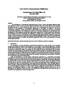
to space limitations, we only present one representative set of data in Figure 1. Packet Reception Percent/LQI Raw Value/RSSI Raw Value
evaluation of the mechanism from two aspects: the end-toend delay and the buffer requirements. Section IV integrates the stream metric into the routing layer design, leading to the second optimization technique. We compare its performance to two state-of-the-art protocols that take into account the unreliable nature of sensor network communication. We demonstrate that, by using the joint optimization, our protocol stack achieves a considerably better EP B value than either of them. At last, we outline related work in Section V and conclude this paper with Section VI.
120 110 100 90 80 70 60 50 40 30 20 10 0 -10 -20 -30 -40 -50 -60 -70 -80 -90 -100
Received Packet Percent Received Packet LQI (averaged per round) Received Packet RSSI (averaged per round)
2 4 6 8 10 12 14 16 18 20 22 24 26 28 30 32 34 36 38 40 42 44 46 48 Experiment Round
Fig. 1. Correlation between the packet receiving ratio and LQI of CC2420 radio at receiver side. At each distance, six rounds of packets are sent from the sender to the receiver.
A. Link Quality Metrics Overview Link quality metrics are used to classify and select links. Prior measurements on link quality reveal that different links have considerably different packet reception properties [30]. One popular model is to treat a link as a bi-directional packet reception probability vector (p, q). However, reception probability is not the only representation of link quality. Recently, another metric, LQI, or Link Quality Indicator, was defined by IEEE standard 802.15.4 [1], and was implemented on the Chipcon CC2420 radio component [7]. The CC2420 radio has been used on MicaZ and Telos nodes. Another interesting link quality indicator is RSSI (Received Signal Strength Indicator), also implemented on the CC2420 radio. In this section, we demonstrate that LQI is closely correlated with packet reception probability, and either of them can be used as the underlying metric of our optimization model. On the other hand, our experiments demonstrate that RSSI is not a satisfactory indicator of link quality, and should not be adopted for link classification. The implementation of LQI, as defined in [1], was that it “may be implemented using receiver ED (energy detection), a signal-to-noise ratio estimation, or a combination of these methods.” The CC2420 radio module implemented LQI based on a sampling of the error rate for the first eight symbols of each incoming packet. This sampling generates a correlation value in the range of [50, 110], followed by a linear conversion of this value to a range of [0, 255], which is the value provided to the user. RSSI is not detailed in the 802.15.4 standard, but it is provided by the CC2420 radio module together with LQI. RSSI is also based on eight symbols, but instead of using the error rate, it uses the average energy level to calculate its value. We carried out a series of experiments with both indoor and outdoor environments during different periods of the day. Due
In this particular experiment, we use a pair of MicaZ nodes, one as the sender and the other as the receiver. We vary the distance from the receiver to the sender from 5f t to 40f t, in steps of 5f t. At each distance, the receiver sends six rounds of packets, with 100 packets in each round. The packet reception ratio, the average LQI and the average RSSI are plotted for comparison. Both LQI and RSSI are calculated in every round. We have three observations. First, we observe a strong correlation between the averaged LQI values and packet reception probabilities at the receiver. Statistical analysis shows that the Pearson’s correlation coefficient is 0.90 between these two variables. Of course, there are still some inconsistencies observed, especially when the received signal is weak. These inconsistencies explain why the Pearson’ s coefficient is not 1.0. Nevertheless, the observed correlation is still quite interesting, since LQI is calculated only from those packets that are received, whereas the packet reception probability takes into account those packets that are dropped. This correlation implies that LQI is a good measurable indicator of the packet reception probability. Second, at each distance, the packet reception probability has a narrow range of variation that is less than 20%. Our additional experiments also exhibit the same property. This observation is consistent with results in the literature [26]. We, therefore, consider the packet reception probability as a relatively stable parameter to classify links. Third, observe that there is a much smaller correlation between RSSI and the packet reception probability. The Pearson’s correlation coefficient is only 0.56 between the packet reception probability and the RSSI value. Furthermore, observe that when the signal is weak, even though there is a considerable variation in the packet loss rate, RSSI does not change appreciably. Therefore, we do not recommend using RSSI as a reliable link quality indicator.
B. The Design of the Lazy Packet Loss Detection We now describe the lazy packet loss detection algorithm. The optimization goal is to minimize EP B. Since this algorithm works in the link layer, we assume a chosen path. For example, we consider the scenario where the source sends 1000 packets to the destination via certain hops. Observe that the amount of meaningful traffic is fixed. Therefore, the optimization goal is equivalent to minimizing the overhead. This goal can also be expressed as maximizing the fraction of non-redundant data packets. We now introduce the path efficiency parameter, η. Formally, for a path with N hops, let U be the total useful traffic delivered in bits, and S be the total amount of bits transmitted from all nodes on this path. We have: UN (1) S Clearly, for a fixed path, η and EP B are inversely proportional. Therefore, for a given path, we want to maximize η. Note that, however, η can not replace EP B when the path is not fixed. For example, one way to maximize η without a given path is to select only strong links (links with high reception probabilities), so that very few packets will be lost. In this case, we obtain a high η value. On the other hand, by only choosing strong links, we are essentially accepting an excessively large number of hops, which increases EP B. The rest of this section optimizes η. First, we consider the upper bound of η. Next, we present the lazy lost packet detection algorithm. At last, we show that the reliable communication model, assumed in this paper, generally achieves a better η than unreliable models. 1) Path Efficiency Upper Bound: We now derive the upper bound of η. A simplified model is shown in Figure 2. η=
Source (p1,q1)
(p2,q2)
Fig. 2.
(p3,q3)
(pn,qn)
Sink
The simplified link model
In this model, we assume a path of n links. Suppose link Li has a forward packet reception probability of pi and a backward packet reception probability of qi . Observe that for a single link, we have: The path efficiency η over a single link cannot be higher than its forward packet reception probability p. The reasoning is intuitive: since useful traffic can only flow forward, if the sender sends N packets, only pN packets can be delivered successfully. Therefore, even if (though this is not practical) the sender knows, without any additional cost, which packets are lost and re-transmits them, an upper bound of p nevertheless holds for η. Next, we consider the path efficiency over multiple links. Suppose the sender intends to send K bits to the destination over n hops. Suppose the total traffic flowing over link Li in both directions is Mi bits. For link Li , we have: ηi =
K ≤ pi Mi
(2)
On the other hand, we know the path efficiency ηpath over n hops is (according to Equation 1): nK ηpath = �n i=1 Mi Let the maximal pi for 1 ≤ i ≤ n be pmax , we have: n ηpath = �n
1 i=1 ηi
n ≤ �n
1 i=1 pi
≤ pmax
(3)
(4)
A tight upper bound on path efficiency η over multiple hops therefore is � nn 1 . Using this bound, we can investigate i=1 pi the available reliable communication models. Surprisingly, few have considered the aspect of efficiency and some intuitive solutions can never approach this bound. Such is the case with the popular timeout-based solution. In a timeout-based solution, the sender generally relies on a timer to control retransmissions. More specifically, if the sender does not receive an acknowledgement from the receiver when the timer fires, it assumes that either the data packet or the acknowledgement is lost. Therefore, it sends the data packet again. This solution is intuitive, elegant and has been proved to be robust in practice. However, despite its merits, we argue that this timeout-based design is inherently less advantageous for sensor networks for efficiency reasons. Specifically, let us consider the number of packets it takes for transmitting one data packet reliably for one hop over a link of reception probabilities of (p, q) using the timeout-based protocol. Since the combined packet delivery success ratio for a round of packet exchanges (i.e., for a pair of data and acknowledgement packets), is pq, the sender is expected to send the data packet 1/pq times before both the data packet and the corresponding acknowledgement packet are delivered successfully. Since the receiver only acknowledges those data packets it receives, it is expected to send 1/pq × p, or 1/q acknowledgements. Let the packet length ratio between the acknowledgement packet and the data packet be λ. The path efficiency η over this pq . As λ → 0, or, if the data packet is link becomes 1+pλ sufficiently large compared to the acknowledgement packet, η approaches pq. Compare this result with Equation 2, as long as the backward link is not perfect, this efficiency value is always smaller than its upper bound. 2) Lazy Lost Packet Detection based Communication: So why does timeout-based design fail to approach the upper bound? Observe that in this design, the key mechanism the sender relies on to detect a packet loss is the acknowledgment packets from the receiver. Unfortunately, the backward link is not perfect, therefore, the sender wastes bandwidth by retransmitting data packets that have been successful. To avoid this problem, therefore, the sender must use additional information, other than the acknowledgements from the receiver, to detect packet losses. In the design described in this section, we use a combination of two techniques, overhearing and sequence number counting, to achieve this purpose. We present three aspects of the new communication model: lazy loss detection, implicit acknowledgement, and path efficiency analysis. The basic mechanism is shown in Figure 3.
Packet 1 overhearing
Packet 1 Packet 1 Packet 2 Packet 2 Packet 3 lost
Ask for retransmission of packet 3
Packet 4 arrives, node B detects lost packet Packet 3 overhearing
Packet 3 retransmitted
Packet 6 overhearing
Packet 6
Node A
Packet 5
Node B
Packet 3 Packet 4 Packet 5 Packet 6
Node C
Fig. 3. This example shows the basic principle of lazy loss detection. At each node, packets are sent out in order, although packets may not be received in order. In this example, A sends out 6 packets in total, and packet 3 is lost when first sent from A to B. B then detects this packet loss after receiving a following packet using sequence number counting, and asks A to retransmit it. Packet 3 is then retransmitted.
Lazy Loss Detection In lazy loss detection, the sender does not employ any timeout mechanism. Rather, the detection of lost packets is delayed to the moment when the receiver gets another packet from the sender. For example, in Figure 3, the loss of packet 3 is not detected until B receives packet 4 from node A. We therefore call this loss detection lazy. The receiver then recovers the lost packets by sending retransmission request packets (RRPs). Since the link from B to A is also not perfect, it may take multiple RRPs to inform A of the lost packet. Therefore, B should periodically resend RRPs, with an interval larger than the round-trip time, until it recovers the lost packet. Obviously, to maintain the correct sequence of packets, we enforce that new packets received by B during this period should be temporarily buffered. Implicit Acknowledgement To respond RRPs, a node must buffer the lost packets. Hence, a node deletes a packet it sent out earlier only when it decides that this packet has indeed been received by the receiver. In practice, the sender relies on implicit acknowledgements. These acknowledgements come from two sources. First, based on the broadcasting nature of wireless links, A can usually overhear the packets sent out by B to downstream nodes. Such overhearing is the first source of implicit acknowledgement That is, once A overhears a packet it sent out earlier being relayed, it can safely delete it from its buffer. For example, in Figure 3, node A can delete packet 1 after it overhears it sent by node B. Second, observe that RRPs can also serve as acknowledgements, as long as RRPs for different lost packets are kept in order. That is, once B decides that a packet has been lost, B should stop relaying new packets, and immediately switch to sending RRPs. When A receives a RRP, it can decide that 1) all packets prior to this lost one must have been successfully received and 2) it should resend the requested (lost) packet. RRPs therefore serve as
implicit acknowledgements. For example, in Figure 3, when B sends RRPs to A regarding the lost packet 3, A decides that previous packets must have been received by B, and can safely delete them from the buffer. Observe that some techniques presented here, such as the packet sequence number counting and the implicit acknowledgement, work only if A continues to send packets to B. For the last few packets in a stream, the sender should either switch to sender-timeout mechanism for packet-loss detection, or it can send additional dummy packets to the receiver. The dummy packets should assume higher sequence numbers, so that the receiver can correctly diagnose potential packet losses. Path Efficiency Analysis We now analyze path efficiency η in the lazy communication model. We define λ as the length ratio between a RRP packet and a data packet. For one link, if the first packet transmission is successful, which has a probability of 1 − p, there are no retransmissions needed. Otherwise, when the receiver detects a packet loss, it sends a request for retransmission. For a link with a delivery ratio of (p, q), the number of RRP s, after a packet loss, conforms to a geometric distribution with parameter pq, and the average number of RRP s sent is 1/pq. On the sender side, since it only responds to those RRP s it receives, the average number of retransmissions for a lost data packet is 1/p. Therefore, the path efficiency is: η=
pq 1 = 1/p + (1 − p)λ/pq q + (1 − p)λ
(5)
The interesting fact regarding Equation 5 is that if the length of data packets is sufficiently large compared to the length of RRP s, or, if λ → 0, η → p. Remember that p is the upper bound for efficiency over a single link. Therefore, we have shown that lazy packet loss detection overcomes the disadvantage of timeout-based mechanisms and approaches the path efficiency upper bound. Additionally, this result indicates that it is beneficial to use various techniques, such as data aggregation, to increase the length of data packets and decrease λ. We can also easily get the expected EP B value over this link: λ 1 1−p 1 + )= + λ (6) p pq p pq EP B represents energy consumption. We demonstrate that once this metric is incorporated into the routing layer design, it can significantly improve the path energy efficiency of data streams (which we call the stream model. EP B = p × 1 + (1 − p) × (1 +
C. Why Reliable Packet Delivery is Important So far, we have assumed our communication model to be reliable. In this section we explain why. We present a comparison between three communication models on path efficiency over multiple hops: our new model (denoted stream), the timeout-resend model (denoted timeout), and the best effort, non-reliable data communication model (denoted noack). For the end-to-end path efficiency, we have:
N
ηstream = �N i=1
qi +(1−pi )λ pi qi
ηtimeout = �N
N
i=1 ηnoack =
1+pi λ pi qi
p1 · p2 · · · pn · N 1 + p1 + p1 · p2 + · · · + p1 · p2 · · · pn−1
(7)
(8) (9)
For an intuitive understanding of their differences, assume the link quality p over different links can be approximated by p˜, and q approximated by q˜. Indeed, such an approximation is highly simplified, and we shall take into account quality reception variations in Section III-A. In the simplified case, we have: ηstream =
p˜q˜ q˜ + (1 − p˜)λ
(10)
p˜q˜ 1 + p˜λ
(11)
ηtimeout = ηnoack =
(1 − p˜) · p˜N · N 1 − p˜N
(12)
These results show one critical difference between the best effort communication model (Equation 12) and the reliable communication model (Equation 10,11): the path efficiency of the best effort model is relevant to the number of hops, whereas the path efficiency of the reliable model is not. Therefore, the best effort communication model is not scalable to long paths. This fact is even more intuitive if we make a further simplification by enforcing that λ → 0 and N → ∞. We get: ηstream → p˜ (λ → 0)
(13)
ηtimeout → p˜q˜ (λ → 0)
(14)
ηnoack → 0 (N → ∞)
(15)
III. U NDERSTANDING THE P ERFORMANCE OF THE S TREAM C OMMUNICATION M ODEL We now present a detailed investigation on the performance of communication model, which we call the stream communication model. We analyze performance from three aspects. First, we study path efficiency through empirical experiments, and validate the performance advantages of the new approach. Next, we analyze end-to-end delay, and validate our results using simulations. At last, we analyze buffer size requirements. A. Empirical Validation of the Communication Model To compare the path efficiency in realistic settings, we used MicaZ nodes to test our communication model. In the experiment, sixteen nodes (labeled 1 to 16) were placed in an indoor hallway. The experiments were carried out at midnight to avoid external interference. The output power level of each node was set to be −7dBm. In the experiment, each node first sent periodic beacons to neighbors to determine the packet reception probability. This process took 2000 packets for each node over a period of 100 seconds. Then, node 1 sent out 3200 packets, hop by hop, to node 16. We enforced that nodes relay the packets sequentially, that is, node 1 sent packets to 2, 2 to 3, etc, at a rate of 2 packets per second. We deliberately chose a low rate to avoid any potential interference, so that the effect of unreliable links can be isolated from that of congestion. Each packet had a payload of 29 bytes, so the overall useful traffic was approximately 100K bytes. We implemented the three different communication models mentioned previously and ran this experiment using each of them separately. Each node logged the number of transmissions, retransmissions, requests for retransmissions, and acknowledgements into its flash. These data were collected after the experiments. The results presented here are based on the analysis of these data. First, we determine the link qualities connecting these nodes. The result is plotted in Figure 4. Note that we only plot link qualities between nodes adjacent to each other.
0.99
This result shows that as the packet travels over many hops, the communication efficiency of the best effort communication model approaches 0! This fact also implies that virtually any conventional design that primarily relies on end-to-end loss recovery techniques can not be ported to sensor networks, due to scalability issues. Arguably, sensor networks represent a new paradigm for communication where sometimes it is difficult to motivate reliable communication. For example, data may be aggregated along the path. The network may indeed tolerate a certain amount of packet losses without significantly affecting the aggregate. However, for the system to scale, the fraction of delivered packets should remain finite and representative of the original pool, which means that a certain degree of reliability is needed to prevent end-to-end communication efficiency from dropping below a certain minimum with an increased hop count.
0.97
0.99
0.59 0.61
0.29 0.99
0.93 0.55
Node 16
0.89
6 .9 0 8 .9 0 0 .9 9
No de 1 0 .9 7
0.99
0.90 0.56
0.96 0.96
0.98 0.97
0.99 0.82
0.94 1
0.29 0.86
0.94 0.51
0.96
Fig. 4. This figure shows the positioning of 16 nodes and the links that connect them, represented by the packet reception probabilities. Links connecting non-neighboring nodes are not plotted for clarity.
We observe several well-known phenomena in wireless communication, such as the existence of link asymmetry and weak links. These phenomena have been reported in prior literature. Based on link quality, we can calculate the expected packet transmission rounds for the stream communication model. The actual packet numbers fit the predictions very well, as shown in Figure 5. There are slight differences between the predictions and the actual measurements in Figure 5, for two reasons. First,
16000
1
Predicted Retransmission Experimental Retransmission Predicted Request for Retransmission Experimental Request for Retransmission
14000
Stream Model Timeout Model Best Effort Model
0.9 0.8 Efficiency up to this Link
Packet Number
12000 10000 8000 6000
0.7 0.6 0.5 0.4 0.3
4000 0.2 2000
0.1
0
0 1
2
3
4
5
6
7
8
9
10 11 12 13 14 15
1
2
3
4
5
Link Number
Fig. 5. This figure compares the predicted and experimental data traffic. The former is calculated based on the analysis of the communication model, and the latter is measured in the experiment.
link quality may change slightly over time. Second, in our implementation, the sender switches to timeout-based packet delivery to ensure reliability at the end of the stream. Both factors lead to slight performance deviations, but Figure 5 demonstrates that these deviations are small and the predictions are still quite accurate. We also compare the efficiency of the stream communication model to the other two models. We plot the results in Figure 6. The path efficiency is calculated based on experimental data. The efficiency for a particular link refers to the accumulated path efficiency from link 1 to this link, as calculated based on the logged data. For example, observe that link 10 corresponds to an efficiency of 0.75 for the stream model, meaning that as data flow from link 1 to 10, the overall efficiency of these ten links is 0.75. Also observe that because of the poor quality of link 2 ((0.51, 0.29) in the experiment), all three communication models experience a considerable decrease in terms of efficiency at link 2. The third observation is that we have similar results as the analysis in Section II-C: the best-effort communication model does not scale with path length and the stream communication model outperforms the other two models considerably. B. End-to-End Delay Analysis To derive the end-to-end delay, observe that this delay contains multiple random variables conforming to different distributions. For example, both the time it takes to detect a packet loss and the number of RRP s sent after the detection of a lost packet conform to geometric distributions, whereas the number of hop-wise delivery failures for a packet from the source to the sink conforms to a binomial distribution. Despite the fact that it is quite difficult to obtain the accurate statistical distribution of the end-to-end delay, it is relatively easy to give an estimate of the expected end-to-end delay. In practice, this parameter is very useful. We derive an estimate of end-to-end delay for two types of traffic: periodic traffic and Poisson traffic. We also validate our analysis using
6
7
8
9
10 11 12 13 14 15
Link Number
Fig. 6. This figure compares the efficiency of three different transport services: stream model, timeout-resend model and best-effort model.
simulations. We do not use empirical data due to the fact that in order to maintain precise time synchronization, which is necessary for calculating the end-to-end delay, current sensor networks protocols employ periodic data exchanges to cope with clock drifts. Such periodic packet exchanges incur a nontrivial traffic overhead and lead to unexpected interference, both of which we want to avoid. Therefore, it is hard to measure precise packet delays without having side-effects on link quality due to interference. Moreover, our simulations also allow us to use a much larger traffic volume to get more precise distribution curves. We first analyze the end-to-end delay for periodic traffic. Consider a path with N hops. Let the delivery latency at each hop be Tl . Let the source generate data packets at a fixed interval, Td . We assume Tl � Td . Suppose the timeout for RRP s is Ta . A packet sent over a link with a reception probability (p, q), has a probability of 1 − p of being lost. One must then wait for a new packet to be successfully transmitted, so that the lost packet can be detected. On average, it takes 1/p new packets before one packet can be successfully delivered. After the lost packet is detected, it takes on average 1/pq RRP s to recover the packet. Therefore, the total expected delay over one hop can be approximated by Tl + (1 − p)( Tpd + Ta pq ). For a path with N links, the end-to-end delay can be estimated as: Delay =
N �
[Tl + (1 − pi )(
i=1
Td Ta + )] pi pi q i
(16)
The analysis for Poisson traffic is quite similar. We model the packet flow as a Poisson process with parameter λ. Therefore, the expected time period for 1/p new packets to be generated is 1/pλ. The end-to-end delay can then be estimated as: Delay =
N � i=1
[Tl + (1 − pi )(
Ta 1 + )] pi λ pi q i
(17)
Both Equations 18 and 17 only model the expected hop delay of the first hop, and then extend this approximation to the remaining hops. Therefore, these results are somewhat sketchy. However, through simulations with different parameters, we find that Equations 18 and 17 indeed provide quite accurate predictions regarding the average end-to-end delay. In the simulation validation, we use the same link quality data set as in Figure 4. All other parameters are set strictly according to MicaZ’s technical specifications. The bandwidth of MicaZ’s CC2420 radio is 250kbps, therefore, the time to transmit one packet is roughly 0.001s. We set the timeout parameter for generating RRP packets to be 0.01s, which is sufficient for one round of packet exchanges. The end-to-end delay distribution from the simulation is plotted in Figure 7. We also plot the theoretical predication of the expected delay, 2.877s, based on Equation 18, along with the average end-toend delay calculated from simulation results. 25
Periodic Traffic Poisson Traffic Predicted Average Delay = 2.877s Periodic Traffic Average Delay = 3.179s Poisson Traffic Average Delay = 3.167s
Packet Percentage (%)
20
15
10
5
0 0-1
1-2
2-3
3-4 4-5
5-6
6-7
7-8
8-9 9-10 10-11 11-1212-1313-1414-1515-1616-17
End-to-End Delay (second)
Fig. 7.
The Distribution of End-to-End Delay
As observed in Figure 7, our earlier theoretical prediction on the average end-to-end delay fits the simulation results with an error of approximately 10%. This error is attributed to the analysis procedure earlier: we simplified the problem by extending the average delay for the first hop to the whole path, while in practice, a packet loss could cause cascading effects, therefore increases the end-to-end delay. We also briefly compare the end-to-end delay of the stream communication model with other communication models. For the best-effort model, it is trivial in that each successfully delivered packet has the minimal delay. For the timeoutbased model, we assume the most generic case in which the sender uses a timer to decide whether a packet it sent has been successfully received. If the timer expires at Ta and no acknowledgement packet is received, the sender retransmits the packet. Therefore, we can easily get the expected end-toend delay for the timeout-based model as: N � 1 [Tl + ( − 1)Ta ] Delay = p i i=1
(18)
Following the settings in Figure 4, the expected end-to-end delay is approximately 70.54ms, which is much smaller than
the stream model. The reason is that in the stream model, the sender relies on subsequent packets to detect potential packet losses. The experiment settings in Figure 4 feature a relatively low data rate, therefore introducing a longer end-to-end delay. C. Buffer Requirement Analysis We now analyze buffer requirements. We consider this problem: given a set of links, what is the appropriate buffer size to avoid packet losses? Although it is much more complex to model the exact relationship between the buffer size and the loss rate, it is usually sufficient to provide a lower bound (i.e., how large the buffer should be to avoid packet losses with high probability). We shall answer this question in this section. There are two requirements that must be satisfied to ensure that packet losses should not occur. First, packet losses should be detected in time before the packet is deleted from the buffer, and second, lost packets should be recovered. Each issue turns out to be a constraint in the model. First, in order to detect lost packets in time, we consider the instant when one packet gets lost. This packet is buffered by the sender until the buffer is full. Then, the oldest packets in the buffer are dropped since we enforce that the buffer is FIFO. During this period, if at least one packet sent after the lost packet is received, then the receiver can detect the packet loss based on sequence number counting. Therefore, as long as the buffer holds enough packets such that at least one packet following the lost packet can be received, the lost packet should be detected. Put in another way, the probability that a packet loss is left undetected is equivalent to the probability that none of the sequence of packets following the lost packet is successfully received before the lost packet is deleted from the buffer. Consequently, for a buffer size of N and a link with a reception probability of (p, q), the probability of a packet loss detection failure is (1 − p)N . In practice, we want this probability to be sufficiently small, for example, less than 10−3 . Therefore, we have: (1 − p)N < 10−3
⇒N >−
3 log10 (1 − p)
(19)
Second, we also need to enforce that lost packets can be recovered. Consider a period of T and a fixed data generation interval of Td , we know TTd packets are to be transmitted. packets are expected to be lost. Since Among them, (1−p)T Td recovering one packet requires on average 1/pq rounds of RRP s, therefore, recovering one packet takes an expected period of Tpqa . Over the period of T , at most TaT/pq packets can be recovered. Since the number of recovered packets must not be smaller than the number of lost packets, therefore, we have: (1 − p)T T > Ta /pq Td
⇒
Td 1−p > Ta pq
(20)
Interestingly, the buffer size does not appear in this constraint, instead, this result implies that both p and q should not be too small. For example, in our earlier experiment, the data rate was 2 packets per second and the timeout was 10
milliseconds. Therefore, TTad = 50. This constraint therefore enforces that 1−p pq < 50. All communication links in the earlier experiment satisfied this constraint. Above all, Equation 19 appears to be the most relevant constraint that the buffer size of each node should satisfy. We use simulations to validate this claim. For simplicity, we enforce that p = q in all cases, and simulate different p values. We plot the relationship between the packet loss ratio and the buffer size from simulations in Figure 8. 100
p/q=0.5/0.5 p/q=0.6/0.6 p/q=0.7/0.7 p/q=0.8/0.8 p/q=0.9/0.9
90
Data Packet Loss Probability
80
p/q=0.5/0.5 Bound = 14 p/q=0.6/0.6 Bound = 10 p/q=0.7/0.7 Bound = 8 p/q=0.8/0.8 Bound = 6 p/q=0.9/0.9 Bound = 4
70 60 50
A. Spanning Tree Routing Structure Optimization
40 30 20 10 0
Fig. 8.
model presented in Section II-B.2 with the spanning tree routing protocol by taking into account link quality variations. The rest of this section is organized as follows. First, we describe in detail the optimization procedure. Next, as a preparation for the comparison and analysis, we present a brief overview of two related path selection methods that appeared in recent literature. Both of them also have taken into account the effect of path quality, though their path quality metrics are different. At last, we compare these three approaches and analyze our results. We use EP B as the primary comparison metric. The comparison results show that the stream communication model achieves a considerably higher energy efficiency than the other two approaches. We believe the performance improvement is primarily attributed to our joint optimization technique across the link layer and the routing layer.
1
2
3
4
5
6
7 8 9 10 11 12 13 14 15 16 17 18 19 20 Buffer Size (Packet Number)
The Relationship between the Buffer Size and the Data Loss Rate
In this simulation, we still use 15 links. We calculate the theoretical prediction (we call them bounds in Figure 8) on buffer size for each link quality setting. These predictions are circled on the X axis at their corresponding positions in this figure. Observe that generally the predictions work quite well. We indeed observe 1 − 5% packet loss even when the predicted buffer size is allocated. Part of the reason is that when multiple lost packets are detected simultaneously, it may take too many rounds of RRP s to recover them, causing the following packets from upstream nodes not to be buffered. To make the problem tractable, our model does not take this effect into account, therefore, slightly larger buffer size should be allocated to reduce packet losses in practice. An interesting observation concerning Figure 8 is that normally, the required buffer size is indeed low. For example, even with quite unreliable links (0.5/0.5), the buffer size requirement is merely 16 packets. Hence, our design is spaceefficient, making it suitable for resource constrained sensor nodes. We also briefly compare the buffer requirement of the stream communication model to other communication models. For the best-effort model, it trivially requires a buffer space of only one packet. For the timeout model, if the timer has a much higher firing rate than the data packet arriving rate, as is the case in our experiment, one packet is almost guaranteed to be received by the next node before the next data packet arrives. Therefore, the buffer requirement is also negligible. IV. ROUTING L AYER O PTIMIZATION In this section, we present the routing layer optimization technique. Specifically, we integrate the stream communication
The optimization of spanning tree routing has two phases: a link estimation phase where each node independently estimates its link quality to immediate neighbors by exchanging packets, and a selective flooding phase where each node obtains its parent node as well as its path cost to the base station. In the first phase, each node broadcasts a fixed number of packets and records the number of successfully received packets from its neighbors. Each node then exchanges this information with neighbors, thereby filling its neighbor table with both outward and inward links with link quality indicators (p, q). In the second phase, the base station initializes a selective flooding procedure to build a weighted routing tree. In the beginning, the base sets the path cost to itself to 0. All other nodes consider the path cost to the base as infinitely large. The base sends out its current path cost to its neighbors. To handle possible packet losses, it rebroadcasts this information multiple rounds. Once one neighbor receives such a packet, if the path cost contained in the packet is smaller than its current path cost, it recalculates its path cost to the base by adding the received path cost, for example, from a node V with a link quality (p, q), with a stream metric cost corresponding to this link, calculated from Equation 6. This node also records V as its parent node. It rebroadcasts its updated path cost after a short waiting period, to avoid congestion. Similarly, it rebroadcasts the update multiple times. Meanwhile, this node records all packets sent by its neighbors, thereby maintaining the path cost information of its neighbors. After the second phase, each node maintains a path cost to the base station through its parent node. By following the parents, one node can reach the base station. We shall next compare the effectiveness of this approach to related approaches in the literature. B. Related Approaches In this section, we give a brief overview of two related path selection approaches that appeared in the recent literature. They are the geographic routing based path selection as
TABLE I S IMULATION S ETTINGS
18
Stream Path Selection ETX Path Selection GF Path Selection Hybrid Path Selection
16
Manchester 50 bytes 55 dBm 1m 200 m 10-25m
14 Average EPB (unit)
Radio FSK Encoding -7 dBm Frame Transmission Medium Path Loss Exponent 3 P LD0 Noise Floor -105 dBm D0 Deployment Configuration Area Height 200 m Area Width Node Number 1000 Range Modulation Output Power
20
12 10 8 6 4 2
100 90
Cumulative Distribution (%)
80 70 60 50 40 30 20 Stream based Path Selection ETX based Path Selection Optimized GF based Path Selection Hybrid Path Selection
10 0 0.5
2.5
4.5
6.5
8.5
10.5 12.5 14.5 16.5 18.5 20.5 22.5 24.5
Energy Per Bit (EPB)(unit)
Fig. 9. The CDF of EPBs for different metrics. The CDF is plotted based on the analysis of all 1000 nodes.
C. Performance Comparison We set up the simulation to reflect realistic communication behavior of sensor networks. We use the radio model in [31], which models many realistic radio features, such as the existence of the transitional region, radio irregularity, and antenna directionality, among others. In our simulation, we
0 100
150 200 250 Area Size (Width/Height)
Fig. 10.
300
Impact of Area Size
16
Stream Path Selection ETX Path Selection GF Path Selection Hybrid Path Selection
14 12 Average EPB (unit)
presented in [18] and a high-throughput metric based path selection as presented in [8]. The authors of [18] compared multiple path selection indicators in the context of geographical forwarding and concluded the metric P RR × distance product achieves the best performance. Here, for a pair of nodes U and V , P RR stands for the packet reception probability of V for packets from U . Distance stands for the distance advanced towards the destination by node V . Node U computes the metric P RR × distance among all its neighbors and selects the maximal one as the best next neighbor. For complete derivations, please refer to [18]. The authors of [8] proposed another metric ET X (the expected number of data transmissions required to send a packet over a link), defined as 1/pq for a link with quality (p, q). [8] did not optimize a spanning tree, instead, it integrated ET X with the DSR routing algorithm. If we consider the base station in the spanning tree as the source node in the DSR routing algorithm, we are able to optimize the spanning tree using the ET X metric based on the approach provided in [8].
10 8 6 4 2 0 800
1000
Fig. 11.
1200 1400 Number of Nodes
1600
Impact of Density
use this model as the radio layer. For a detailed description of the radio model, please refer to [31]. We set the parameters of the radio strictly according to the technical specifications of the MicaZ radio module. There are, of course, several adjustable parameters of the CC2420 radio on the MicaZ nodes, such as the output power. In this case, we adjust the parameters consistently with our earlier experiments. The complete simulation setup is shown in Table I. In the simulation, we assume that nodes are randomly deployed in a square area. The default number of nodes is 1000, and the default area size is 200m × 200m. One node is positioned at (0, 0) to serve as the base station. After nodes form a spanning tree structure, we apply different optimization procedures, and calculate the EP B value for each node. We assume the energy consumed for transmitting one bit over one hop at the default power level −7dBm is one unit. We plot the results for four different mechanisms: ET X based Path Selection in [8]; Optimized GF Path Selection in [18]; Stream based Path Selection as proposed in this paper; Hybrid Path Selection, which uses the ET X metric to select paths and uses the stream communication model to deliver packets. The reasoning behind the last path selection is that we want to isolate the optimization effect of the routing layer. In each of the following experiments, fifty rounds of sim-
Stream Path Selection ETX Path Selection GF Path Selection Hybrid Path Selection
-10
-8
Fig. 12.
-6 -4 Output Power Level (dBm)
-2
0
Impact of Output Power Level
20
Stream Path Selection ETX Path Selection GF Path Selection Hybrid Path Selection
18 16
12 10 8 6 4 2 0 0
1
2
3
4
5
Shadowing Standard Deviation
Fig. 13.
Impact of the Shadow Standard Deviation
ulations are carried out and the averaged values from these rounds are used. A confidence interval of 95% is used where applicable. Figure 9 compares the EP B distributions of the four aforementioned path selection mechanisms. A lower EP B means a better energy efficiency. We observe that the stream based path selection performs the best, followed by the hybrid path selection, then the optimized GF path selection, and at last, the ET X based path selection. As described earlier, one EP B unit stands for the energy consumption for a transmission of one bit over one hop at the output power level of −7dBm. We also study the impact of two adjustable parameters: the area size and the node density. Figure 10 plots the impact of the area size, where node density is the same across different settings. The average EP B for all nodes is used for comparison. Observe that the stream based path selection consistently performs the best. This figure and the three following figures also have the confidence level plotted. In Figure 11, we vary the node density. The number of nodes varies from 800 to 1600, and the area is kept at 200m×200m. An interesting observation is that as the density increases, EP B slightly decreases. This is quite intuitive since increased density implies better paths may exist, which leads to a decreased energy cost. Another consistent observation is
Reception Probability (%)
Average EPB (unit)
14
that the stream based path selection performs the best. Figure 12 considers the effects of different output power levels. The area size is 200m × 200m. Notice that the unit in this figure still means the energy consumption for transmitting one bit using an output power level of −7dBm. The energy consumption values of other output power levels are scaled to this unit. Interestingly, we observe that by increasing the output power level, the energy consumption grows considerably, even though we did observe reduced path length in terms of hops and better connectivity. Figure 13 considers the effect of a transitional region, in which the link quality changes abruptly. The existence of a transitional region has been repeatedly reported in the recent literature [26], [30], [31]. In the radio model we use, we are able to tune the parameter σ, the shadowing standard deviation, to adjust the width of the transitional region: a smaller σ leads to a narrower transitional region. In this experiment, we change the value of σ from 0, where the transitional region does not exist, to 5, where a very wide transitional region appears. The σ value of MicaZ nodes is approximately 3.8 [31]. We observe from the results that, generally, a larger transitional region leads to better performance in terms of EP B. This indicates that, interestingly, a smart use of the highly varied links in the transitional zone can improve the performance. In fact, this is because a wider transitional region provides more links to choose from. However, we cannot make the assertion that choosing more links in the transitional region always leads to better performance. A counterexample is observed in the following experiment. 100 90 80 70 60 50 40 30 20 10 0
Reception Probability 1
4
14
7
10 13 16 19 22 25 28 31 34 37 40 43 46 49 Distance(m)
All Neighbor Pairs Parent-Child Neighbor Pairs using Stream Metric Parent-Child Neighbor Pairs using Optimized GF Metric
12 Percentage(%)
Average EPB (unit)
38 36 34 32 30 28 26 24 22 20 18 16 14 12 10 8 6 4 2 0
10 8 6 4 2 0
1
4
7
10 13 16 19 22 25 28 31 34 37 40 43 46 49 Distance (m)
Fig. 14.
Neighbor Selection Comparison
In the next experiment, we consider this interesting problem: exactly what is the relationship between the link choice and the energy efficiency? For example, does choosing more links in the transitional region generally lead to better performance? To answer this question, we study three distributions: the distribution of distances of all neighbor pairs, the distribution of distances of neighbor pairs that have parent-child
relationship using the stream based path selection, and the distribution of distances between neighbors that have parentchild relationship using the optimized GF path selection. We know that the stream based path selection performs better than the optimized GF path selection, so is this a result of choosing more links in the transitional region? As a comparison, we also plot the transitional region based on the radio model. Observe that the transitional zone spans roughly from 10m to 30m. Comparing the two sub-graphs in Figure 14, the first important observation is that links inside the transitional zone are obviously preferred compared to other links in both path selection policies. This is consistent with the observations made in [18]. The second observation is even more interesting: the optimized GF path selection uses considerably more links in the transitional zone than the stream based path selection. We believe the reason is that the optimized GF path selection is too aggressive in terms of selecting far away links with poor connectivity. Combine this fact with our earlier results, we know that choosing links in the transitional region too aggressively actually degrades the overall energy efficiency. 100 90
Cumulative Distribution (%)
80 70 60 50 40 30 20 Stream Path Selection ETX Path Selection GF Path Selection
10 0 1
2
3
4
5
6
7
8
9 10 11 12 13 14 15 16 17 18 19 20 Hop Count
Fig. 15. Distribution of Hop Counts for Different Path Selection Mechanisms
The last experiment studies the distribution of hop count numbers using different path selection metrics. The hop count metric is the conventional path length parameter. Since the hybrid path selection leads to the same path length as the ET X based path selection, we only need to compare three metrics. The results are shown in Figure 15. Observe that the stream based path selection generally leads to the shortest paths, followed by the ET X based path selection and the optimized GF path selection. One very interesting, yet somewhat counter intuitive observation about Figure 15 and Figure 14 is that the optimized GF path selection selects more links in the transitional region (which are expected to be more distant) than the stream based path selection, yet it still has longer paths. The reason is that the stream based path selection incorporates a flooding process to build the routing structure, yet GF only uses local information to make path selection choices. Therefore, although the optimized GF approach does choose distant links more aggressively, such links may not lead the packets in the
globally right direction. Therefore, the paths in the optimized GF path selection are relatively longer. D. Conclusion Based on the comparison results, we can decrease EP B by using the stream metric in the routing layer. Of course, one serious limitation of the spanning tree routing structure is that it can only support a limited number of base stations, while the optimized GF mechanism presented in [18] can handle more generalized peer-to-peer communication patterns. Nevertheless, since many applications indeed use only a few base stations, we believe our study is quite applicable to these real systems. Furthermore, we plan to extend the stream based communication model to more generalized, peer-to-peer communication patterns in our future work. V. R ELATED W ORK Research on radio properties [6], [30] indicates that the wireless links between low power sensor devices are extremely unreliable. Specifically, Woo [26] points out the existence of three distinct data reception regions within a radio range: full connected, transitional and disconnected regions. In the transitional region, the reception of data becomes highly varied. Meanwhile, it is observed that, in realistic systems, the radio qualities are severely affected by the multi-path effect, reflection, diffusion, scattering and ground attenuation [10], [22], [12]. To achieve reliability over unreliable links, many protocols have been designed, evaluated and implemented [8], [18], [17], [21], [27]. Some protocols regard the reliability in data delivery as a main design goal. For example, RMST [21] (Reliable Multi-Segment Transport) tracks packet fragments so that receiver-initiated requests, using NACK control packets, can be satisfied when individual pieces of an application payload get lost. Another work is the transport layer design of Wisden [27]. The transport layer of Wisden shares some features of RMST and uses overhearing in the same way as our stream communication model. In addition, robust data delivery [9] simultaneously sends packets along multiple paths at the expense of increased communication overhead. Our work is different from these approaches in the sense that we achieve communication efficiency and reliability, simultaneously. Recently there also have been some protocols designed to address both reliability and congestion, simultaneously. Among them are CODA [24] and ESRT [17]. Both protocols are more focused on how to reduce congestion through various techniques. Specifically, CODA uses a sampling of the channel to determine whether the channel is currently congested, and if it is, nodes decrease the traffic allowed. Alteratively, ESRT monitors the current network state based on the congestion conditions in the network. Such conditions guide ESRT to adjust the reporting frequency of the source node to maintain event-to-sink reliability dynamically. The topic of efficiency has been considered less frequently in the recent literature. Representative protocols include Fusion [11] and a revised geographical forwarding proposed
in [18]. Both protocols discussed possible enhancements on efficiency. In Fusion, the main topic is how to leverage various congestion-control mechanisms to increase efficiency. In [18], the authors studied how to minimize the energy spent in geographical routing, therefore increasing efficiency as well. Neither of them, however, presented a systematic study of the relationship between efficiency and link quality, nor did they propose any new communication models. Therefore, our work is quite novel in this aspect and provides significant insight on communication efficiency. The study of communication efficiency falls into a larger research topic: energy efficiency, where solutions are even more diversified. Lower power microcontrollers [2], radio circuits and antenna designs [7], [16] significantly reduce energy consumption in data delivery at the hardware level. Media Access Control [15], [23], [29] reduces the network contention, hence reduces the number of retransmissions. Sensing coverage protocols [25], [28], [20], [5] provide surveillance to a certain geographic area with a minimal energy budget. Data aggregation techniques [14], [19] reduce the number of messages sent while still distributing information an application requires. Data cache techniques [4] are also designed for applications where multiple sinks coexist and use caching to update and distribute data to leaf nodes at the minimally requested rate. Cross-layer designs [13], [20] coordinate the operations of the physical, medium access control (MAC), and routing layers together to achieve a better efficiency than what can be achieved by individual protocols. Since these protocols achieve energy efficiency from different perspectives, we consider them orthogonal and complimentary to our work. VI. C ONCLUSIONS In this paper, we have studied the problem of communication efficiency based on a quantitative modeling of wireless link unreliability. We followed a joint-optimization process that considers both the link layer lost packet recovery and the routing layer path selection. Our contributions are twofold. First, in the link layer, we present a lazy lost packet detection and recovery technique that proves to be especially useful in terms of improving efficiency. Second, we develop and use a stream metric for path selection in the routing layer. Compared with other state of the art path selection approaches, our joint optimization considerably decreases Energy Per Bit. Our simulation and implementation results demonstrate the correctness of our approach, and give us fundamental insight into the efficiency aspect of sensor network communication over unreliable links. ACKNOWLEDGMENTS We would like to thank Marco Zuniga at the ANRG group of USC for sending us the source code of their radio model. We also would like to thank the anonymous reviewers for their insightful comments. The work reported in this paper was supported in part by the National Science Foundation
grants EHS-0208769, CSR-0509233, and NETS-0435060, and by MURI grant N00014-01-1-0576. R EFERENCES [1] IEEE standard 802.15.4 2003. [2] ATmega128 Specification, Atmel Corporation, available at www.atmel.com/acrobat/doc2467.pdf. [3] M. Batalin et al., “Call and response: Experiments in sampling the environment,” in ACM Sensys, 2004. [4] S. Bhattacharya et al., “Energy-Conserving Data Placement and Asynchronous Multicast in Wireless Sensor Networks,” in MobiSys, 2003. [5] M. Cardei et al., “Energy-efficient target coverage in wireless sensor networks,” in IEEE Infocom, 2005. [6] A. Cerpa et al., “Statistical model of lossy links in wireless sensor networks,” in IPSN, 2005. [7] CC2420 Product Information and Data Sheet, chipcon, avaiable at http://www.chipcon.com/. [8] D. D. Couto et al., “A high-throughput path metric for multi-hop wireless routing,” in ACM Mobicom, 2003. [9] D. Ganesan et al., “Highly resilient, energy efficient multipath routing in wireless sensor networks,” in Mobile Computing and Communications Review, 2002. [10] T. He et al., “An Energy-Efficient Surveillance System Using Wireless Sensor Networks,” in MobiSys, 2004. [11] B. Hull et al., “Techniques for mitigating congestion in sensor networks,” in ACM Sensys, 2004. [12] V. Kottapalli et al., “Two-tiered Wireless Sensor Network Architecture for Structural Health Monitoring,” in Proc. of the Intl. Symp. on Smart Structures and Materials, 2003. [13] R. Madan et al., “Cross-layer design for lifetime maximization in interference-limited wireless sensor networks,” in IEEE Infocom, 2005. [14] S. Madden et al., “TAG: A Tiny Aggregation Service for Ad-Hoc Sensor Networks,” in Operating Systems Design and Implementation, 2002. [15] J. Polastre and D. Culler, “Versatile Low Power Media Access for Wireless Sensor Networks,” in SenSys, 2004. [16] J. M. Rabaey et al., “PicoRadio Supports Ad Hoc Ultra-Low Power Wireless Networking,” Computer Magazine, vol. 33, no. 7, 2000. [17] Y. Sankarasubramaniam et al., “Esrt: Event-to-sink reliable transport in wireless sensor networks,” in ACM Mobihoc, 2003. [18] K. Seada et al., “Energy efficient forwarding strategies for geographic routing in lossy wireless sensor networks,” in ACM Sensys, 2004. [19] N. Shrivastava et al., “Medians and Beyond: New Aggregation Techniques for Sensor Networks,” in SenSys, 2004. [20] M. L. Sichitiu, “Cross-layer scheduling for power efficiency in wireless sensor networks,” in IEEE Infocom, 2004. [21] F. Stann and J. Heidemann, “Rmst: Reliable data transport in sensor networks,” in IEEE SNPA, 2003. [22] R. Szewczyk et al., “An Analysis of a Large Scale Habit Monitoring Application,” in SenSys, 2004. [23] T. van Dam and K. Langendoen, “An Adaptive Energy-Efficient MAC Protocol for Wireless Sensor Networks,” in SenSys, 2003. [24] C.-Y. Wan et al., “Coda: Congestion detection and avoidance in sensor networks,” in ACM Sensys, 2003. [25] X. Wang et al., “Integrated Coverage and Connectivity Configuration in Wireless Sensor Networks,” in SenSys, 2003. [26] A. Woo et al., “Taming the Underlying Challenges of Reliable Multihop Routing in Sensor Networks,” in SenSys, 2003. [27] N. Xu et al., “A wireless sensor network for strucutral monitoring,” in ACM Sensys, 2004. [28] T. Yan et al., “Differentiated Surveillance Service for Sensor Networks,” in SenSys, 2003. [29] W. Ye et al., “An Energy-Efficient MAC Protocol for Wireless Sensor Networks,” in IEEE INFOCOM, 2002. [30] J. Zhao and R. Govindan, “Understanding packet delivery performance in dense wireless sensor networks,” in ACM Sensys, 2003. [31] M. Zuniga and B. Krishnamachari, “Analyzing the transitional region in low power wireless links,” in IEEE SECON, 2004.