Model Projection - UCL Computer Science

Model Projection: Simplifying Models in Response to Restricting the Environment Kelly Androutsopoulos1 David Binkley2 David Clark1 Nicolas Gold1 Mark Harman1 Kevin Lano3 Zheng Li1 1

University College London, Malet Place, London, WC1E 6BT, UK. 2 Loyola University Maryland, Baltimore, MD 21210-2699, USA. 3 King’s College London, Strand, London, WC2R 2LS, UK.

ABSTRACT This paper introduces Model Projection. Finite state models such as Extended Finite State Machines are being used in an ever increasing number of software engineering activities. Model projection facilitates model development by specializing models for a specific operating environment. A projection is useful in many design-level applications including specification reuse and property verification. The applicability of model projection rests upon three critical concerns: correctness, effectiveness, and efficiency, all of which are addressed in this paper. We introduce four related algorithms for model projection and prove each correct. We also present an empirical study of effectiveness and efficiency using ten models, including widely–studied benchmarks as well as industrial models. Results show that a typical projection includes about half of the states and a third of the transitions from the original model.

Categories and Subject Descriptors D.2.2 [Software Engineering]: Design Tools and Techniques

General Terms Algorithms, Theory, Experimentation

Keywords Model Projection, Extended Finite State Machines, Slicing

1.

INTRODUCTION

Both automatically and manually generated state-based models find many applications in software engineering. For example, they are often constructed by model checkers [8] and built by engineers in the telecommunications and embedded systems sectors [9, 10, 25]. They are also used in modelling notations such as the UML [28], which draws heavily on state-based modelling [27], and are widely used for specifying discrete-event control devices, such as automated manufacturing systems (AMS) [30]. A great deal of engineering effort is directed towards the design of an organisation’s models. As a result, it is common for models to be reused. One such scenario arises when control models are reused within a device that offers a restricted operational environment. For example, the ‘basic model’ car air conditioning system may not offer the climate control functionality found in more luxurious models. It would be wasteful to specify different models for each potential car Permission to make digital or hard copies of all or part of this work for personal or classroom use is granted without fee provided that copies are not made or distributed for profit or commercial advantage and that copies bear this notice and the full citation on the first page. To copy otherwise, or republish, to post on servers or to redistribute to lists, requires prior specific permission and/or a fee. ICSE11, May 21-28 2011, Waikiki, Honolulu, HI, USA Copyright 2011 ACM 978-1-4503-0445-0/11/05 ...$10.00.

configuration. Rather, there is typically a single controller for the entire product line [3]. In this situation, model projections, specialized to the particular environment, are useful as they avoid producing bloated controllers that implement unused functionality. The design of models typically occurs earlier in the overall development process than coding where the cost of errors is, in general, higher. This makes it important to have powerful and flexible tools for model analysis. Model projection facilitates such analysis in much the same way that techniques such as program transformation and program slicing assist with code level analysis [29, 16, 32]. Figure 1 presents an example of model projection in which a vending machine allows a user to insert coins and vends tea with options of large cups, small cups, sugar, and double sugar. Consider redeploying this controller in an environment where the ‘sugar’ button is disabled, and thus in an environment in which the event Sugar() never occurs. The projection removes all states and transitions (shown in dashed grey) unreachable by event sequences in the restricted environment. This causes the state Sugar to become unreachable and subsequently the state Double Sugar, because it is only reachable from the state Sugar. When these states and their associated transitions are projected out of the model, only the black elements remain. Model projection can also be used to facilitate property verification by reducing the complexity of a model and thus making analysis more efficient. Consider the production cell example used in the industrial case study of a German metal processing plant [26]. In this system, metal blanks enter the system on a feed belt and are conveyed via a table by robot arms to one of two presses. Assume that we want to prove that the feed belt motor is off if there is a blank on the belt and a blank on the elevating rotating table. Call this property P . It turns out that property P only concerns two sensors and one actuator of the model. To prove that P holds in the original model requires consideration of a state space having over 3,000 states. However, only four events affect P (s1on, s1off, s3on, s3off). A model projection produced by ignoring all other events has only four states and eight transitions. This substantial reduction in controller size means that P can be verified to hold in all states directly. As shown in Section 4, this implies that P holds in the original model. With these applications and others, the applicability of our approach depends upon both correctness and the reduction achieved in reasonable time. Therefore, this paper concerns the theoretical and empirical underpinnings of model projection as formalized in Section 2. Section 3 then introduces four progressively more precise (and more expensive) model projection algorithms. This is followed in Section 4 by proofs of correctness for the four algorithms. Finally, Section 5 investigates the effectiveness and efficiency of our approach in terms of the reduction achieved on a set of ten models (including standard benchmarks and real world models).

insertsmallcups(n)[n>0]/k1=k1+n; insertlargecups(n)[n>0]/k=k+n; EXIT

Coin()[t+250]/price=p;

dispose()

Idle Tea() [k>1 && s==1]/ k=k-1;

Coin()

smallcup()/ s=2;

insertsmallcups(n) [n>0]/ k1=n;

Coins Inserted

largecup()/ s=1;

Tea() [k>1 && s==1]/ k=k-1;

Cancel() Tea() [k1>1 && s==2]/ k1=k1-1;

Cancel()

Coin() [t+25>=price && price>0]/ s=0;t=0;

Tea() [k1>1 && s==2]/ k1=k1-1; largecup()/ s=1;

Sugar()

smallcup()/ s=2;

Cancel() Tea() [k1>1 && s==2]/ k1=k1-1;

MoreSugar()

Sugar

Tea() [k1==1 && s==2]/ k1=k1-1;

Coin() Tea() [k==1 && s==1]/ k=k-1;

Tea() [k==1 && s==1]/ k=k-1;

2.

Tea() [k1>1 && s==2]/ k1=k1-1;

Tea() [k1==1 && s==2]/ k1=k1-1; Tea() [k==1 && s==1]/ k=k-1;

No Small Cups

No Large Cups

Coin()

Coin()

MODEL PROJECTION DEFINITION

This section first introduces some notation and terminology related to the particular models focused on in this paper: Extended Finite State Machines (EFSMs). It then formalizes the notion of a projection for EFSMs. Definition 1 (Extended Finite State Machines (EFSMs)) An EFSM M is a tuple (S, T, A, Si ) where S is a set of states, T is a set of state to state transitions, A is an event alphabet (a set of events), and Si is the set of initial states. A transition t ∈ T has a label lbl(t) of the form e()[g]/a, where e ∈ A, g is a boolean guard, written in an unspecified condition language, and a is an action, written in an unspecified command language. All parts of the label are optional. Only when the guard evaluates to True can the transition be taken. An omitted guard is assumed to be True. For transition t, source(t), target(t), guard(t), trigger(t), and action(t) are used to refer to t’s source state, target state, boolean guard, trigger event, and action, respectively. An EFSM M takes as input a sequence of events E ∈ A∗ . Each event includes, in addition to the event name, a list of formal parameters that are passed values from the external environment with the event. A transition’s action commonly updates the store and may produce output events, which need not come from A. Finally, if two transitions share the same source state, the same trigger event, and their guards can be simultaneously True, then M is a non-deterministic EFSM; otherwise, it is deterministic. A completely specified EFSM includes, for every state, a transition triggered by every event in the event alphabet A. Since completeness can often obscure the true nature of an EFSM, as a convention EFSMs are often presented with certain transitions left implicit. A common interpretation for implicit transitions is a self transition. In effect the event is consumed by having the state machine stutter (repeat) the same state without any effect other than consuming the event. The following definition formalizes the event sequences that do not require stuttering. Definition 2 (Implicit Transition Free Event Sequence) For EFSM M = (S, T, A, Si ), an input event sequence E ∈ A∗ is referred to as implicit transition free if M takes no implicit transitions when presented with E. Such an event sequence is also referred to as stutter-free. For a set of event sequences X, itf(M, X) denotes the implicit transition free subset of X: itf(M, X) = {E ∈ X | M takes no implicit transitions when processing E}.

Coin()

Double Sugar

Tea() [k1==1 && s==2]/ k1=k1-1;

largecup()/ s=1;

smallcup()/ s=2;

insertlargecups(n) [n>0]/ k=n;

Figure 1: Illustrative example: model projection for a simple vending machine. The complete vending machine includes both the dashed grey and black elements. The projection, for reuse in an environment where sugar is unavailable (the ‘sugar’ button is disabled), includes only the black elements of the model. The states and transitions concerned with providing sugar are projected out of the model. The projection is faithful to all other (sugar free) interactions with its environment.

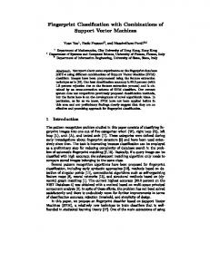
basicProjection(EFSM M = (S, T, A, Si ), Ignore Event Set I) Let M 0 = (S 0 , T 0 , A, Si ) where S 0 = {s0 ∈ S | ∃ path p = s · · · s0 ∈ T ∗ ∧ s ∈ Si } ∧ ∀ t ∈ p, trigger(t) 6∈ I T 0 = {t ∈ T | source(t) ∈ S 0 ∧ target(t) ∈ S 0 } in M 0 = (S 0 , T 0 , A − I, Si ) Figure 2: The basic model projection. Given a set of events to ignore, denoted I, the projection of EFSM M preserves M ’s behavior when placed in an environment that does not generate events from I. The resulting set of event sequences, formalized by the following filter, is used to define model projection. Definition 3 (Event Sequence Set Filter) Sequence-set Filter function fi(X, I) = {E ∈ X | E ∩ I = ∅} where E ∩ I denotes the intersection of the set of events in E with I. Definition 4 (Model Projection) A Model Projection of EFSM M = (S, T, A, Si ) for ignore set I is a reduced EFSM M 0 that is semantically indistinguishable from M on all event sequences from fi(A∗ , I). For a projection to be semantically indistinguishable as required by the definition, it must preserve the behavior of the original machine. There are two aspects to this semantic requirement: what behavior is preserved and over what set of event sequences it is preserved. The first of these, “what behavior is preserved” is formalized by Definition 9 in Section 4. Informally, the behavior includes the variable values computed at each state. The second aspect of the semantic requirement considers the set of event sequences over which the semantics is preserved. Two options are considered: the strong semantic requirement and the weak semantic requirement. Under the strong requirement, behavior is preserved on all sequences in fi(A∗ , I), while for the weak requirement, behavior is preserved only for the stutter free sequences of fi(itf(M, A∗ ), I). Thus the weak requirement does not require matching behavior on event sequences for which the EFSM implicitly consumes an event. Rather, it restricts this requirement to event sequences where the behavior of M is explicitly defined. Figure 2 presents the definition of a basic projection of an EFSM, which is illustrated by the example in Figure 1. In Section 4 we

prove that the implementation of basicProjection shown in Figure 3 satisfies the strong semantic requirement. Furthermore this algorithms removal of states and transitions can facilitate further simplifications. Thus three additional algorithms go beyond the basic projection and consider simplifying the state machine using constant propagation and state merging. The most aggressive of the state merging algorithms satisfies only the weak semantic requirement.

3.

ALGORITHMS

This section describes four model projection algorithms that represent differing performance/precision tradeoffs. Model projection has several possible implementation strategies. For example, one could build a projection by adding necessary elements to an initially empty model. Alternatively, one could remove elements from the model being projected. The initial implementation follows the later approach. To do so, it recasts the notion of program slicing [34] to the EFSM domain. However, this recasting differs from previous work on slicing state-based models [17, 21, 23, 24, 33], which transplant concepts from the program slicing [34] in an attempt to incrementally adapt program-slicing concepts and techniques. These differences are considered further in Sections 5.3 and 6. For much of its history, dependence analysis has typically been applied to programs, but there has been a recent increase in the theory and practice of dependence analysis for models, and in particular state-based models [1]. Indeed, it has been argued [15] that all descriptions, whether they be specifications, models, or other descriptions, will have a tendency to become executable over time, making such descriptions more likely to become the subject of techniques associated with program analysis, such as dependence analysis and slicing. The recent interest in dependence analysis for state-based models makes it timely to consider whether notions of slicing, hitherto defined for programs, remain appropriate when transplanted into the paradigm of models. This paper argues that the notion of slicing needs to be generalised to one of model projection for considering models both EFSMs and otherwise. Specifically, the ‘slicing criterion’ and algorithms for slicing will need to take account of model-specific characteristics. The recasting of slicing used to implement model projection provides a more natural slicing approach by providing a more natural way to specify the slicing criterion: an environment-based slice is taken with respect to an ignore set I. As shown in Sections 4 and 5, environment-based slicing correctly and effectively implements model projection. This achieves a long standing goal in program slicing of defining the slicing criteria in terms of higher level concepts [14, 34]. The remainder of this section first introduces the slicing algorithm basicSlice and then three extensions that incorporate constant propagation and 2 different state mergings. Figure 3 presents basicSlice. Given as a slicing criterion an ignore set I, basicSlice computes a slice by deleting all transitions whose trigger event corresponds to events in the ignore set. Then it removes all states and their transitions that are no longer reachable from an initial state. The reduced model is a basicProjection as defined in Figure 2. Figure 1 shows the basicSlice produced for the Vending Machine example using the ignore set I = {Sugar()}. The first extension to basicSlice, Algorithm A2 is shown in Figure 4, incorporates constant propagation. Algorithm A2 further reduces the projection’s size by replacing a constant-valued variable by its value throughout the machine. When a guard is updated, it may simplify to False; thus the corresponding transition (and perhaps its target state) can be removed. The algorithm implements a simple flow-insensitive constant propagation algorithm in which variables are mapped to values in a flat lattice [12]. Initially vari-

basicSlice(EFSM M = (S, T, A), Ignore Event Set I) { M0 ← M delete from T 0 all transitions t where trigger(t) ∈ I while ∃ state s with no incoming transitions do remove s and all transitions t where source(t) = s return M 0 } Figure 3: Algorithm A1 : basicSlice. Basic algorithm for computing an environment-based slice. ables that appear as formal parameters of an event labelling a transition are assigned the value ⊥ (non-constant) because they receive an unknown value from the environment. All other variables v are initialized to > (uninitialized). The assignments that label the transitions are then taken into account. If the right-hand side of the assignment evaluates to a constant then the value of the left-hand side variable is replaced with the meet of the constant and the variable’s present value. Otherwise, the value is replaced with ⊥. In addition to constant propagation, two state merging algorithms are used to further reduce the size of a projection by combining groups of states that have identical semantics. The right-equivalent merging algorithm extends an algorithm of Ilie et al. [19] to EFSMs. R-equivalence equates to bisimulation for deterministic state

SliceCP (EFSM M , Ignore Event Set I) { M 0 = basicSlice(M, I) constantPropagation(M 0 ) return M 0 } constantPropagation(EFSM M = (S, T, A, Si )) { 8 < ⊥ if v is used as a formal parameter of an input event in a transition label σ ¯ = λ v. : > otherwise foreach t ∈ T foreach assignment “v = exp” ∈ action(t) let x = result of evaluating exp using σ ¯ in update(¯ σ , v, x) deleteUnTriggerableTransitions(M 0 , σ ¯) } deleteUnTriggerableTransitions(EFSM M = (S, T, A, Si ), abstract store σ ¯) { while ∃ t ∈ T where guard(t) evaluates to False using σ ¯ remove t from T while ∃ s ∈ S with no incoming transitions do remove s and all transitions t¯ where source(t¯) = s } where update(¯ σ , v, x) replaces v’s value in σ ¯ with σ ¯ (v) u x using the following meet operation: >u>=> >uC =C >u⊥=⊥ C uC =C C u C 0 = ⊥(C 6= C 0 ) C u⊥=⊥ ⊥u⊥=⊥ Figure 4: Algorithm A2 : Constant Propagation removes transitions whose guard is always False.

SliceM erge (EFSM M , Ignore Event Set I) { M 0 = basicSlice(M, I) constantPropagation(M 0 ) R-mergeEquivalentStates(M 0 ) if only satisfying the weak semantic requirement then G-mergeEquivalentStates(M 0 ) } R-mergeEquivalentStates(EFSM M = (S, T, A, Si )) { while ∃ States s1 , s2 ∈ S such that R-equivalent(s1 , s2 ) replace s1 and s2 with s, where s has as its outgoing (and self-) transitions a copy of those of s1 , and incoming transitions the union of those of s1 and s2 . } R-equivalent(States s1 , s2 ) { if finalState(s1 ) ∧ not finalState(s2 ) or not finalState(s1 ) ∧ finalState(s2 ) return false else return true iff ∀ t ∈ T · source(t) = s1 ⇒ ∃ t0 : T · source(t0 ) = s2 ∧ trigger(t0 ) = trigger(t) ∧ action(t0 ) = action(t) ∧ guard(t0 ) ≡ guard(t) ∧ target(t0 ) ∼ target(t) 0 ∀ t ∈ T · source(t) = s2 ⇒ ∃ t : T · source(t0 ) = s1 ∧ trigger(t0 ) = trigger(t) ∧ action(t0 ) = action(t) ∧ guard(t0 ) ≡ guard(t) ∧ target(t0 ) ∼ target(t) // Where s1 ∼ s2 means the targets are the same state, or one is s1 and the other s2 . } G-mergeEquivalentStates(EFSM M = (S, T, A, Si )) { For a set of transitions T , triggers[T ] denotes the set of triggers of the transitions of T . Function metric(g) denotes the number of states removed by merging groups in g into single states: Σs∈g (| s | −1) where | s | denotes the size of set s. possibleGroups = {ss ∈ 2S | | ss | ≥ 2 ∧ (∀ t ∈ T · source(t) ∈ ss ∧ target(t) ∈ ss ⇒ action(t) = skip) ∧ ( (triggers[{t ∈ T | source(t) ∈ ss ∧ target(t) ∈ ss}] ∩ triggers[{t ∈ T | source(t) ∈ ss ∧ target(t) 6∈ ss}] = ∅)} if possibleGroups 6= ∅ then mergeGroups = {pg ∈ 2possibleGroups | pg 6= ∅ ∧ ∀ state sets ss1 , ss2 ∈ pg · ss1 6= ss2 ⇒ ss1 ∩ ss2 = ∅} bestGroup = g ∈ mergeGroups such that metric(g) is maximal. collapseStates(M, bestGroup) } Figure 5: Algorithms A3 and A4 : Two State Merging algorithms machines. It has a counterpart that merges left-equivalent states. However, this merge is only relevant for non-deterministic EFSMs and is not presently implemented. Merging both R-equivalent and Lequivalent states forms a bisimulation for general EFSMs. The approach, implemented by the function R-mergeEquivalentStates, shown in Figure 5, repeatedly merges pairs of states provided that the two states of the pair are R-equivalent, until no further merging is possible. States s1 and s2 are R-equivalent if, for every transition from s1 , there is a corresponding transition from s2 and vice versa. That is, for each trigger event, the outgoing transitions from the two states are identical in their guards and actions, and have equivalent target states after the merge (i.e., s1 and s2 are considered to be the same state). This transformation preserves the regular expression language (i.e., the set of stutter-free event sequences) accepted by the state machine. The second merging algorithm, G-mergeEquivalentStates, shown in Figure 5, is a more aggressive merge that can yield greater simplification and, as a tradeoff, only preserves the weak semantic requirement. In this function the set possibleGroups includes all

groups (subsets of S) that are eligible to be merged into single states. A group ss can be merged if it has size two or more, all transitions within the group have no actions, and the set of internal triggering events is disjoint from the set of exiting triggering events. The set of internal triggering events includes those events that trigger transitions from a state in ss to another state in ss while the set of exiting triggering events includes those events that trigger transitions from a state in ss to a state outside of ss. While unimplemented, it is possible to relax this requirement and allow the merge, provided that for all events E, the guard conditions of each internal transition triggered by E are logically inconsistent with the guard conditions of all of the exiting transitions triggered by E. If the set possibleGroups is non-empty, then some merging is possible. To determine the best merge, a set of all possibilities mergeGroups is defined. This set includes subsets of possibleGroups that are pairwise disjoint and can thus be merged simultaneously. Finally, the subset that maximizes the number of states removed is chosen. Because this algorithm is exponential in the number of states (which is likely to be the case for any algorithm which considers all possi-

ble candidates for state merging) future work includes considering heuristics for applying G-mergeEquivalentStates. However the empirical study reported in Section 5.3 indicates that, in practice, the run times are reasonable. Figure 6 illustrates the impact of constant propagation and state merging. EFSM A is sliced with respect to ignore set I = {a}. Slicing removes the two assignments to x when it deletes the transitions from s3 → s4 and s5 → s4 . This leaves x with the constant value 1. Constant propagation rewrites the guard x < 2 on the transition from s4 to the final state to “True”, which in turn enables R-merging of states s4 and s5 leading to EFSM B. EFSM C shows the result of R-merging states s1 and s3 . This merge does not require constant propagation; thus the example illustrates both that some merging is possible without performing constant propagation and that constant propagation can enable (additional) merging. If only stutterfree sequences are acceptable then G-mergeEquivalentStates can be used. This merges s1 , s3 and s4 , s5 yielding EFSM D.

4.

A

s2 /x =1

b

Definition 5 (Configurations) Let Σ be the set of all possible stores for an EFSM. For EFSM M = (S, T, A, Si ), a configuration is a pair (s, σ) where s ∈ S is a state and σ ∈ Σ is a store.

s3

Definition 7 (Enabled Transitions) For Status St = (C, E) of an EFSM M = (S, T, A, Si ) where C = (s, σ), transition t is enabled iff source(t) = s, guard(t) evaluates to True when evaluated using σ, and trigger(t) = head(E). The set Enabled(St) denotes the set of all transitions enabled in Status St. The semantics of an EFSM M , is formalized as a Labeled Transition System (LTS). States of the LTS are the statuses of M and transitions of the LTS have the same labels as the transitions of M but extended with an additional label for implicit transitions (see the operational semantics definition below) . The LTS has a labeled step rule which defines legal transitions. A closed system assumption is made in which the status is only changed explicitly by the step rule. The semantics of EFSM M taking enabled transition t is given as an LTS move from Status St1 to Status St2 , denoted t M ` St1 −−−→ St2 . In doing so the store is updated using the LT S

store update function denoted by [[action(t)]]. This single step rule is formalized as follows: Definition 8 (LTS Step − −− →) LT S

For Status St = ((s, σ), E) of EFSM M , taking enabled transition t produces the next status: t ∈ Enabled(St) ∧ σ 0 = [[action(t)]]σ t

M ` ((source(t), σ), E) −−−→ LT S

((target(t), σ 0 ), tail(E))

s4 a/x =5

g

g

b[x