Efficiency Enhancement of Optimized Latin Hypercube Sampling ...

Postprint: Rajabi MM, Ataie-Ashtiani B, Janssen H. 2015. Efficiency enhancement of optimized Latin hypercube sampling strategies: Application to Monte Carlo uncertainty analysis and metamodeling, Advances in Water Resources, 76:127-139.

doi:10.1016/j.advwatres.2014.12.008

Efficiency Enhancement of Optimized Latin Hypercube Sampling Strategies: Application to Monte Carlo Uncertainty Analysis and Meta-modeling Mohammad Mahdi Rajabi 1,*, Behzad Ataie-Ashtiani 1, Hans Janssen 2 1. Department of Civil Engineering, Sharif University of Technology, PO Box 11155-9313, Tehran, Iran. 2. KU Leuven, Department of Civil Engineering, Building Physics Section, Kasteelpark Arenberg 40, 3000 Leuven, Belgium.

*: Department of Civil Engineering, Sharif University of Technology, PO Box 11155-9313, Tehran, Iran; [email protected].

Abstract: The majority of literature regarding optimized Latin hypercube sampling (OLHS) is devoted to increasing the efficiency of these sampling strategies through the development of new algorithms based on the combination of innovative space-filling criteria and specialized optimization schemes. However, little attention has been given to the impact of the initial design that is fed into the optimization algorithm, on the efficiency of OLHS strategies. Previous studies, as well as codes developed for OLHS, have relied on one of the following two approaches for the selection of the initial design in OLHS: (1) the use of random points in the hypercube intervals (random LHS), and (2) the use of midpoints in the hypercube intervals (midpoint LHS). Both approaches have been extensively used, but no attempt has been previously made to compare the efficiency and robustness of their resulting sample designs. In this study we compare the two approaches and show that the space-filling characteristics of OLHS designs are sensitive to the initial design that is fed into the optimization algorithm. It is also illustrated that the space-filling characteristics of OLHS designs based on midpoint LHS are significantly better those based on random LHS. The two approaches are compared by incorporating their resulting sample designs in Monte Carlo simulation (MCS) for uncertainty propagation analysis, and then, by employing the sample designs in the selection of the training set for constructing non-intrusive polynomial chaos expansion (NIPCE) meta-models which subsequently replace the original full model in MCSs. The analysis is based on two case studies involving numerical simulation of density dependent flow and solute transport in porous media within the context of seawater intrusion 1


doi:10.1016/j.advwatres.2014.12.008 in coastal aquifers. We show that the use of midpoint LHS as the initial design increases the efficiency and robustness of the resulting MCSs and NIPCE meta-models. The study also illustrates that this relative improvement decreases with increasing number of sample points and input parameter dimensions. Since the computational time and efforts for generating the sample designs in the two approaches are identical, the use of midpoint LHS as the initial design in OLHS is thus recommended. Keywords: Uncertainty propagation; Monte Carlo simulation; Non-intrusive polynomial chaos expansion; Optimized Latin hypercube sampling. Highlights 

The effect of initial design in optimized Latin hypercube sampling (OLHS) is studied.



Resulting sampling methods are applied to Monte Carlo simulations and meta-modeling.



The comparisons are based on two test cases of seawater intrusion.



Shows that use of midpoints in hypercube intervals as initial design increases the efficiency of OLHS.

1. Introduction The input parameters of many analytical, numerical, geospatial and statistical models in hydrology, hydrogeology and water resources management are prone to uncertainty, resulting either from their inherent stochasticity or from the lack of knowledge about their exact values [1,2]. During the simulation process, the uncertainty in model inputs inevitably propagates through the model and results in uncertainty of the output quantities of interest. Quantifying this propagated uncertainty is known as uncertainty propagation (UP) analysis [3]. UP analysis is a key component of uncertainty quantification and forms the basis for predictive uncertainty analysis, global sensitivity analysis, risk analysis and simulation-optimization under uncertainty. There are a variety of methods for UP analysis, from which the most commonly used method is Monte Carlo simulation (MCS) [4]. MCS is a non-intrusive, sampling-based, numerical method [5], which involves generating a number of samples from the probability density functions (PDFs) that characterize the uncertainty in model inputs, running the model at the set of sampled points, and then using the ensemble of model outcomes to approximate the statistical characteristics and probability distribution of the output quantities of interest [6,7]. MCS often requires a large ensemble of sample points to provide a reliable and stable 2


doi:10.1016/j.advwatres.2014.12.008 estimate of uncertainty [8]. This makes MCS computationally expensive especially when the model itself is computationally demanding. However, the number of sample points required to reach a certain level of accuracy is highly dependent on the efficiency of the sampling strategy. A more efficient sampling strategy requires fewer sample points and hence less simulation time to achieve a specific level of accuracy [9]. The efficiency of a sampling strategy itself depends on the space-filling and non-collapsing characteristics of its resulting sample designs [10,11]. Space-fillingness indicates how evenly the sample points are spread out over the design space. A sampling strategy with inferior space-filling characteristics requires more sample points and hence more deterministic solves to ensure a full coverage of the design space [12,13]. Non-collapsingness insures that the design points do not coincide when projected onto a lower number of dimensions. This coincidence of design points decreases the worth of data contained within the resultant simulations [12,13]. 1.1. Sampling methods for MCS If we look at the timeline of studies involving UP analysis based on MCS in hydrology, hydrogeology and water resources management, we see that earlier studies mostly involve standard (also known as crude or simple) MCS which rely on simple random sampling (SRS). However, several studies have shown that SRS is not an efficient sampling strategy due to its less appealing space-filling and non-collapsing characteristics [6,13-15]. Many attempts have been made during the past decades to introduce more efficient sampling strategies. This has resulted in the introduction of numerous random, quasi-random or deterministic sampling strategies. A widely used example of these methods is Latin hypercube sampling (LHS) [16]. The stratified sampling approach of LHS ensures that the resulting sample designs are non-collapsing and generally more space-filling than SRS [17] and thus, LHS is shown to be more efficient compared to SRS [4,13,15,16,18,19]. There are consequently many recent examples for the use of LHS in hydrology, hydrogeology, and water resources science and management literature and several codes have been developed for UP analysis based on LHS (e.g. REPTool [20,21], PEST-LHS [22] and FEMWATERLHS [23]). However, LHS does not necessarily lead to optimal space-filling designs [24]. A new class of sampling strategies has therefore been proposed in recent years aiming at improving the space-filling characteristics of LHS designs. These so-called optimized Latin hypercube sampling (OLHS) strategies take a LHS design as the "initial design" and then iteratively optimize the location of sample points with respect to a space-filling criterion until 3


doi:10.1016/j.advwatres.2014.12.008 a set of stopping criteria are satisfied [25]. Several studies have illustrated the superior efficiency of OLHS designs compared to SRS and LHS, most notably in cases where UP analysis is based on a small to medium number of simulations (e.g. 101 to 102) [e.g. 13,15,26,27]. Several OLHS strategies have been proposed in the literature, which differ according to their optimization algorithm and the space-filling criterion used as the objective function. Rajabi and Ataie-Ashtiani [15] compared nine OLHS strategies including improved Latin hypercube sampling (IHS) [28]; optimum Latin hypercube (OLH) sampling [29-31]; genetic optimum Latin hypercube (GOLH) sampling [26,31]; three sampling strategies based on the enhanced stochastic evolutionary (ESE) optimization algorithm [27] namely 𝜑𝑝 -ESE which employs the 𝜑𝑝 space-filling criterion, CLD-ESE which utilizes the centered L2-discrepancy (CLD) space-filling criterion, and SLD-ESE which uses the star L2-discrepancy (SLD) space-filling criterion; and three sampling strategies based on the simulated annealing (SA) optimization algorithm [26,27] namely 𝜑𝑝 -SA which employs the 𝜑𝑝 criterion, CLD-SA which uses the CLD criterion, and SLD-SA which utilizes the SLD criterion. They applied these strategies to two test cases involving the numerical simulation of seawater intrusion (SWI) and concluded that the CLD-ESE strategy is the most efficient amongst the evaluated strategies. Further increase in the efficiency of OLHS strategies is currently the subject of much research. 1.2. Meta-modeling in MCS Beside the use of more efficient sampling strategies, MCS can also be accelerated through meta-modeling approaches which involve developing data-driven, physics-free and computationally cheap approximations of the model response [32]. The meta-models then replace the original model in MCS and thereby reduce the computational burden of MCS up to several orders of magnitude depending on the computational time of the original full model [33]. Meta-modeling approaches include the use of radial basis functions (RBFS), neural networks (NNs), support vector machines (SVMs), non-intrusive polynomial chaos expansions (NIPCEs), Gaussian process emulators (GPEs) etc. No matter which of these methods is selected, they all require a training set of simulator runs, which is selected through deterministic or random sampling methods. The number of model simulations required for the generation of an adequate training set is often immensely smaller than the number of model simulations required for the case in which MCS based on the original model is used.

4


doi:10.1016/j.advwatres.2014.12.008 Nevertheless, generating the required training set could still be computationally problematic when dealing with models with extremely high computational demand. When the selection of the training set is based on random sampling, we are faced with a kind of design of experiment problem in which: (1) the training set of points should be chosen so that no prediction is too far from a training point. Thus, the training points should be spread over the input space in which the predictions will be made. (2) We also want this to be true when we project the points into lower dimensions. These considerations imply that the sample design should be space-filling and non-collapsing. Increasing the number of sample points could potentially lead to a more space-filling design. However, this increase involves more deterministic simulations and the computational cost will also increase. Hence, we are faced with the same problem as in the case of MCS, a situation in which a limited number of sample points are computationally affordable and we want a sample design that results in the most accurate estimation of uncertainties through the incorporation of meta-modeling methods in MCS. This gives rise to the importance of sampling efficiency in the generation of the training set for the construction of meta-models, which has been a common topic of research within the meta-modelling community, see for example [9,33-35]. The appealing space-filling and non-collapsing characteristics of OLHS designs imply that OLHS strategies can effectively provide more efficient training sets for the construction of meta-models. 1.3. Study objectives The majority of previous studies regarding OLHS are dedicated to increasing the efficiency of these sampling strategies through the development of new algorithms based on the combination of innovative space-filling criteria and optimization schemes. However, little attention has been paid to the impact of the initial design that is fed into the optimization algorithm, on the efficiency of the resulting sample designs. A review of literature shows that in previous studies, the nature of the initial design in OLHS strategies is often either ambiguous or implicitly described. Nonetheless, we can infer from the available literature that two approaches have been previously used for the selection of the initial design in OLHS strategies. The first approach is the use of random points in the hypercube intervals which we denote here as random LHS. The second approach is to employ midpoints in the hypercube intervals, here referred to as midpoint LHS. The scientific literature has somewhat favored the use of midpoint LHS. Examples include [26] for OLHS strategies based on the SA optimization algorithm, [27] for OLHS strategies based on the ESE optimization algorithm, 5


doi:10.1016/j.advwatres.2014.12.008 and [31] for OLH and GOLH sampling strategies. Instances of the use of random LHS are prevalent in tailored software packages, examples include ‘DiceDesign’ (see [36]) by Franco, Dupuy and Roustant, and ‘lhs’ by [37], both of which are developed for the R open source statistics software, the Matlab toolbox ‘lhsdesign’ (see [38]), and the generator of designs in the JMP statistical software (for general information see [39], and for information about their Monte Carlo design generator refer to [40]). The basic objective of this paper is to compare the effect of using these two approaches (i.e. random LHS and midpoint LHS) for the selection of the initial design that is fed into the optimization algorithm in OLHS strategies, on the efficiency of the resulting sample designs. Note that the computational time and efforts for the generation of the sample design in the two approaches are identical. First, we will compare the space-filling characteristics of the sample designs generated by the two strategies to see if and how the resulting sample designs are affected by the initial design. We will then incorporate the resulting sample designs in MCS for UP analysis and assess the relative efficiency of the two approaches. The sample designs are subsequently employed in the selection of the training set for constructing NIPCE meta-models which subsequently replace the original full model in MCS. So this study deals with both MCS and meta-modeling. We focus our analysis on the CLD-ESE OLHS strategy which was shown by [13,15] to be the most efficient method amongst the set of evaluated OLHS strategies. The two methods for the selection of the initial design in OLHS strategies are applied to case studies involving numerical simulation of density dependent groundwater flow and solute transport resulting from SWI in coastal aquifers. Density dependent SWI numerical models involve solving coupled differential equations that characterize mass and solute transport in porous media, and are well known in the groundwater modeling community for their highly non-linear and non-smooth input-output relationship [41,42]. A number of points should be addressed here to clarify the study objectives and scope. First, a key assumption of LHS and OLHS strategies is that the uncertain inputs are independent from each other, and this is also the case in the current study. When dealing with problems in which the correlation of the uncertain inputs must be considered (such as the uncertain inputs describing a heterogeneous hydraulic conductivity field [43,44]), the generation of sample points could be done by using LHS or OLHS in conjunction with a procedure introduced by [45] to induce a desired rank correlation structure on the resultant design [4, 46]. Second, the concern here is to find an optimal sample design where the number of design points is 6


doi:10.1016/j.advwatres.2014.12.008 determined in advance based on factors such as computational constrains and required level of uncertainty quantification and the entire design is generated at once and not sequentially. 2. Theoretical Background First, we briefly describe the theoretical background of the CLD-ESE sampling strategy. A brief introduction to NIPCEs and the methods used for the estimation of NIPCE coefficients is subsequently given in section 2.2. 2.1. The CLD-ESE OLHS Strategy The ESE optimization algorithm used within the context of the CLD-ESE OLHS strategy consists of two coupled loops, an inner loop and an outer loop. The CLD-ESE sampling strategy obtains an initial design (denoted here by 𝑌0 ) with the required number of sample points which is then fed into the inner loop of the ESE optimization algorithm. The inner loop uses the initial design to generate a number of new designs by element exchanges. The algorithms then evaluate the space-filling characteristics of the generated designs with respect to the CLD criterion, with the intention of finding the best design among them [15,27]. The CLD criterion provides a quantitative measure to assess the deviation of a sampling design from perfectly uniform point density and is defined as [17]: 2

𝑁(𝑌𝑢 , 𝐽𝑦𝑢 ) 𝐶𝐿𝐷(𝑌) = ∑ ∫ | − 𝑉𝑜𝑙(𝐽𝑦𝑢 )| 𝑑𝑢 𝑛 𝑢

(1)

𝐶𝑢

Where 𝑢 is a nonempty subset of the coordinate indices 𝛺 = {1, … , 𝜃}, 𝐶 𝑢 is the |𝑢| dimensional unit cube involving the coordinates in 𝑢, 𝑉𝑜𝑙(𝐽𝑦𝑢 ) is the volume of the subset 𝐽𝑦𝑢 , 𝐽𝑦𝑢 is the projection of 𝐽𝑦 on 𝐶 𝑢 , 𝐽𝑦 is an 𝜃 dimensional interval uniquely defined by 𝑌, 𝑌𝑢 is the projection of 𝑌 to 𝐶 𝑢 , 𝑌 is the set of 𝑛 points {𝑦1 , … , 𝑦𝑛 }, and 𝑁(𝑌𝑢 , 𝐽𝑦𝑢 ) is the number of points of 𝑌𝑢 falling in 𝐽𝑦𝑢 . Smaller CLD values are an indication of more uniform sample designs. The ESE algorithm subsequently decides whether to accept or reject the best design with respect an acceptance criterion as follows [27]: 𝑖𝑓 𝐶𝐿𝐷(𝑌𝑖 ) < CLD(𝑌0 ) ⇒ 𝑌𝑖 = 𝑌𝑡𝑟𝑦 (𝑖. 𝑒. 𝑌𝑡𝑟𝑦 𝑖𝑠 𝑎𝑐𝑐𝑝𝑒𝑡𝑒𝑑) 𝑒𝑙𝑠𝑒 𝑖𝑓 |𝐶𝐿𝐷(𝑌𝑖 ) − 𝐶𝐿𝐷(𝑌0 )| ≦ 𝑇ℎ × random(0, 1) ⇒ 𝑌𝑖 = 𝑌𝑡𝑟𝑦 (𝑖. 𝑒. 𝑌𝑡𝑟𝑦 𝑖𝑠 𝑎𝑐𝑐𝑝𝑒𝑡𝑒𝑑)

7

(2)


doi:10.1016/j.advwatres.2014.12.008 𝑒𝑙𝑠𝑒 𝑌𝑡𝑟𝑦 𝑖𝑠 𝑟𝑒𝑗𝑒𝑐𝑡𝑒𝑑 In Eq. 2, 𝑌𝑡𝑟𝑦 denotes the best design, random (0, 1) is a uniformly distributed random number generated between 0 and 1, and 𝑇ℎ is a threshold. The inner loop iteratively repeats this process by a user supplied number of times, with 𝑌0 replaced by 𝑌𝑖 . Then, the outer loop of the ESE algorithm updates the acceptance criterion and the inner loop restarts the optimization process once again. This continues until the user specified number of iterations for the outer loop is reached [15]. 2.2. The NIPCE meta-model NIPCEs have been extensively used in many scientific disciplines such as structural dynamics [47], heat conduction [48], air pollution dispersion [49], fluid dynamics problems [50] and SWI modeling [51]. The widespread use of NIPCEs as a meta-modeling approach in MCS can be attributed to their transparency, simplicity, strong mathematical basis, ability to handle many probability distribution types and to be used with any second order random process, and the fact that they allow for a fully probabilistic prediction of what the simulator would produce [5,51-53]. NIPCEs decompose the uncertain output quantities of interest into separate deterministic and stochastic components in the form of a series described by the following equation [53-54]: ∞

𝑦 = ∑ 𝛼𝑖 𝜓𝑖 (𝜉)

(3)

𝑖=0

In Eq. 3, 𝑦 is the output quantity of interest and 𝛼𝑖 represents a set of deterministic NIPCE coefficients. In the univariate case, 𝜉 is a random variable with a predefined probability distribution and 𝜓𝑖 is an orthogonal polynomial of order 𝑖 which forms the stochastic component of the NIPCE. In the multivariate situation, 𝜉 is a vector and the polynomial 𝜓𝑖 is a tensor product of the polynomial bases for each component of 𝜉. The optimal choice for the type of orthogonal polynomial used in NIPCEs is dictated by the probability distribution of 𝜉 and is usually selected in accordance with the Askey scheme [55]. For practical reasons, the series in Eq. 3 is often truncated to a limited number of terms. The use of NIPCEs for UP analysis involves two basic steps. First, the deterministic coefficients of the NIPCE for each of the output quantities of interest are estimated. Second, the NIPCE replaces the original model in MCS in order to provide an estimate of the PDF of 8


doi:10.1016/j.advwatres.2014.12.008 the outputs. The statistics describing the uncertainty in model outputs can then be calculated with respect to the PDF of the outputs. In this case, the computational cost associated with UP analysis is mostly transferred to the estimation of the NIPCE coefficients, leaving the subsequent MCS computationally inexpensive [53,56]. After the NIPCEs are built, the type of sampling method used in the framework of the MCS+NIPCE UP strategy is a trivial issue, because NIPCEs are computationally very economic and a very large number of sample points are hence affordable. In this case, due to the large number of simulations, the results converge to the true solution regardless of the sampling strategy. With the use of NIPCEs the mean, variance and Sobol indices of the output quantities of interest are also available in closed-form without the need to perform MCS. There are a number of methods for estimating the coefficients of NIPCEs including the spectral projection methods (which involves the sampling-based and quadrature-based methods) [57,58], the probabilistic (or stochastic) collocation method (PCM) [59], the gradient-based method also known as collocation method coupled with sensitivity derivatives [60], and the regression method [61]. All of these methods require a training set of simulator runs. The PCM, gradient-based and quadrature-based spectral projection methods use a predetermined number of training points which are commonly selected through deterministic methods. On the other hand, the sample-based spectral projection method and the regression method often (but not necessarily) involve random sampling for the generation of the training set [62,63]. The number of training points is user defined but often constrained to a minimum value for the spectral projection and regression methods. In this study, the coefficients of NIPCEs are estimated by the regression method because: (1) we are focusing on random sampling for the generation of the training set, (2) the regression method converges faster in terms of the number of model evaluations compared to the projection method [64,65], and (3) the regression method is a very flexible, transparent, understandable and easy to code method for the estimation of NIPCE coefficients. The regression method involves choosing a set of 𝑞 training or regression points in the probability space of the random input variable(s) (𝜉 (𝑘) , 𝑘 = 1, … , 𝑞) through deterministic or random sampling methods. These regression points are then used to perform 𝑞 simulations of the model which we denote by 𝑦(𝜉 (𝑘) ) ( 𝑘 = 1, … , 𝑞). The NIPCE coefficients are subsequently estimated by solving the following minimization problem [56]: 9


doi:10.1016/j.advwatres.2014.12.008 2

𝑚𝑖𝑛 {∑𝑞𝑘=1[𝑦(𝜉 (𝑘) ) − ∑𝑑𝑖=0 𝛼𝑖 𝜓𝑖 (𝜉 (𝑘) )] }

(4)

Eq. 4 can be solved by optimization algorithms such as pattern search [66] and simulated annealing [67]. For the general multivariate case with 𝑚 variables, the number of coefficients to be estimated is 𝑁𝑐𝑜𝑒𝑓𝑓 = (𝑚+𝑑 ). It has been widely suggested that the number of sample 𝑑 points must be greater than 𝑁𝑐𝑜𝑒𝑓𝑓 [68]. Note that Eq. 4 can also be written as a system of 𝑞 nonlinear equations which could then be solved by using the Levenberg-Marquardt [69] algorithm. In this study we use this latter approach to estimate the NIPCE coefficients. 3. Test Cases We will try to answer the objective questions of this study by examining two synthetic test cases of SWI in coastal aquifer systems described in [15]. Both test cases involve density dependent flow and solute transport in porous media which is basically modeled by the following coupled differential equations that characterized mass and solute transport [70,71]: (𝜌𝑆𝑜𝑝 )

𝜕𝑝 𝜕𝜌 𝜕𝑐 𝑘𝜌 + (𝜀 ) − 𝛻. [( ) . (𝛻𝑝 − 𝜌𝑔)] = 𝑄𝑝 𝜕𝑡 𝜕𝑐 𝜕𝑡 𝜇𝑓𝑙𝑢𝑖𝑑

𝜕(𝜀𝜌𝑐) + 𝛻. (𝜀𝜌𝜈𝑐) − 𝛻. [𝜀𝜌(𝐷𝑚 𝐼 + 𝐷). 𝛻𝑐] = 𝑄𝑝 (𝑐 ∗ − 𝑐) 𝜕𝑡

(5-a) (5-b)

Where 𝜌 is fluid density, 𝑆𝑜𝑝 is specific pressure storativity, 𝑝 is fluid pressure, 𝑡 is time, 𝜀 is aquifer volumetric porosity, 𝑐 is solute concentration (mass solute/mass fluid), 𝑘 is solid matrix permeability, 𝜇𝑓𝑙𝑢𝑖𝑑 is fluid dynamic viscosity, 𝑔 is gravitational acceleration, 𝑄𝑝 is the fluid mass sink or source, 𝜈 is average fluid velocity, 𝐷𝑚 is apparent molecular diffusion coefficient, 𝐼 is identity tensor, 𝐷 is mechanical dispersion tensor, and 𝑐 ∗ is the concentration of solute in the source fluid. The simulations are carried out using the USGS SUTRA finite element numerical code [70]. No assumptions have been made regarding the input/output relationships and the mathematical properties of the system except that the noise is assumed to be identical for two simulation runs with the same inputs (i.e. the simulator is assumed to be deterministic). Therefore, we expect the basic conclusions of the study to be generally applicable to UP studies. The two test cases are briefly described in the following paragraphs and further details can be found in [15].

10

Frame 001  27 Jun 2014MM,  Example: Multi-Zone 2D Postprint: Rajabi Ataie-Ashtiani B,Plot Janssen

H. 2015. Efficiency enhancement of optimized Latin hypercube sampling strategies: Application to Monte Carlo uncertainty analysis and metamodeling, Advances in Water Resources, 76:127-139.

doi:10.1016/j.advwatres.2014.12.008

Monitoring point

(a)

Numerical grid

Constant fluid source (𝑄𝑖𝑛𝐻 , 𝐶𝑄𝑖𝑛 ) 𝐻

0.1 m

0.1 m

Sea boundary

Inland boundary

Frame 001  27 Jun 2014  Example: Multi-Zone 2D Plot 1m

0m 0m

Impermeable boundary

2m

Specified pressure (𝑃 = 𝜌𝑠𝑤 . 𝑔. 𝑑𝑒𝑝𝑡ℎ, 𝐶𝑠𝑤 ) (b) Concentration (kg/kg): Concentration

0.035 0.03 0.025 0.02 0.015 0.01 0.005

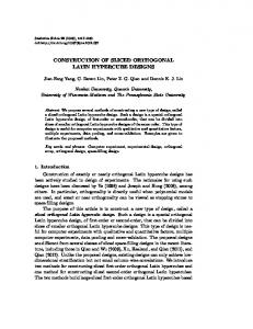
Fig. 1 The Henry problem [72]: (a) problem domain, boundary conditions, numerical grid and monitoring point, (b) concentration in the steady state solution

11


doi:10.1016/j.advwatres.2014.12.008 Table 1 Input parameter values for the Henry problem [15] Parameter Permeability (𝑘𝐻 )

Value

Unit

Uncertain: log-normal (μ=1.020408×10-9, σ2=9.5×10-19)

m2

0.0

m

Longitudinal and transverse dispersivities Freshwater inflow (𝑄𝑖𝑛𝐻 )

Uncertain: log-normal (μ=0.06, σ2=0.0008)

kg/s

0.35

---

1.88571×10-5

m2/s

1×10-3

kg/m.s

0.0

kg/kg

0.0357

kg/kg

Density of freshwater

1000

kg/m3

Density of seawater

1024.99

kg/ m3

Porosity Molecular diffusion Viscosity Freshwater solute concentration (𝐶𝑖𝑛𝐻 ) Salt concentration of seawater (𝐶𝑆𝑊 )

The Henry problem [72] illustrated in Figs. 1a and 1b, involves a two dimensional cross section of a confined coastal aquifer system. The problem domain is rectangular and the top and bottom boundaries are assumed to be impermeable. Seawater intrudes the system from the seaward boundary on one side of the problem domain and freshwater flows into the system from the inland boundary on the other side. The problem domain is homogeneous and fully saturated. Here, the aquifer is initially filled with freshwater. During the simulation period, seawater begins to intrude the freshwater system by moving under the freshwater from the sea boundary, while freshwater flows over the seawater in the section and discharges at the sea boundary. The simulation is continued long enough for the concentration distribution to reach steady state. The input parameter values used in numerical simulations of the Henry problem are specified in Table 1. The permeability of the aquifer (𝑘𝐻 ) and the total constant fresh-water inflow on the inland boundary (𝑄𝑖𝑛𝐻 ) are assumed to be the uncertain input parameters. The uncertainty of 𝑘𝐻 and 𝑄𝑖𝑛𝐻 are characterized by lognormal distributions described in Table 1. Note that it is common to employ log-normal distributions to represent uncertainty of permeability in relatively homogeneous aquifers [73]. It has also been illustrated in previous studies (such as [74]) that the uncertainty in recharge rate can be characterized by log-normal distributions [51]. The output quantities of

12


doi:10.1016/j.advwatres.2014.12.008 interest are pressure and salt concentration values in an arbitrary chosen monitoring point illustrated in Fig. 1a.

(a)

Freshwater recharge: Constant fluid source (𝑄𝑖𝑛𝐼𝑠 , 𝐶𝑄𝑖𝑛 ) 𝐼𝑠

202014 m  Example: Multi-Zone 2D Plot Frame 001  27 Jun

~6.7 m m

+5 m 5m

Sea boundary

-100 m

Impermeable boundary 0m

400 m

500 m

800 m

Specified pressure (𝑃 = 𝜌𝑠𝑤 . 𝑔. 𝑑𝑒𝑝𝑡ℎ, 𝐶𝑠𝑤 )

Monitoring point Numerical grid

(b) Concentration (kg/kg): Concentration: 0.005 0.01 0.015 0.02 0.025 0.03 0.035

Fig. 2 The radial island problem [60,63]: (a) problem domain, boundary conditions, numerical grid and monitoring point, (b) concentration in the steady state solution

13


doi:10.1016/j.advwatres.2014.12.008 Table 2 Input parameter values for the radial island problem [15] Parameter

Value

Unit

Horizontal permeability

Uncertain: log-normal (μ=5×10-12, σ2=1×10-24)

m2

Vertical permeability

Uncertain: log-normal (μ=5×10-13, σ2=1×10-26)

m2

Longitudinal dispersivity for horizontal flow

Uncertain: log-normal (μ=10, σ2=8)

m

Longitudinal dispersivity for vertical flow


m

Transverse dispersivity


m

2.3766×10-5

Freshwater inflow (𝑄𝑖𝑛𝐼𝑠 ) Porosity


kg/ m2.s

---

1.0×10-9

m2/s

1×10-3

kg/m.s

0.0

kg/kg

0.0357

kg/kg

Density of freshwater

1000

kg/m3

Density of seawater

1024.99

kg/ m3

Molecular diffusion Viscosity Freshwater solute concentration (𝐶𝑖𝑛𝐼𝑠 ) Salt concentration of seawater (𝐶𝑆𝑊 )

The second test case is a circular island surrounded by seawater, based on [70,75] (see Figs. 2a and 2b). This problem was adapted for UP analyses by [15]. It is assumed that due to a long-term drought, the island's aquifer is filled with seawater and the water table has declined to sea level. This is the initial condition of the model and we simulate the post-drought conditions in which a freshwater lens is formed due to seawater being flushed out of the aquifer system by constant rainwater recharge. The simulations are continued until the system reaches steady state and the equilibrium fresh groundwater lens is established [75,76]. The aquifer system is assumed to be homogeneous but anisotropic. The radial symmetry of the problem allows it to be represented by a two-dimensional cross section that stretches from the seaward boundary to the axis passing through the center of the island. The boundary representing this axis and the bottom boundary are assumed to be impermeable. Freshwater recharge enters the aquifer system from the island surface. The input parameters of the model are given in Table 2. It is assumed that there are six uncertain input parameters, namely porosity, horizontal permeability, vertical permeability, longitudinal dispersivity for horizontal flow, longitudinal dispersivity for vertical flow, and transverse dispersivity. The 14


doi:10.1016/j.advwatres.2014.12.008 statistical characteristics of the purely hypothetical PDFs characterizing the uncertainty of these input parameters are presented in Table 2. The output quantity of interest is the salt concentration in an arbitrary chosen monitoring points illustrated in Fig. 2a. 4. Results and Discussion Here, we denote the CLD-ESE sampling strategy with the initial design generated by random LHS as CLD-ESE (rand), and the CLD-ESE sampling strategy with the initial design generated by midpoint LHS as CLD-ESE (mid). The two sampling strategies are compared first by studying the space-filling characteristics of their resulting sample designs and then by incorporating them in MCS based on the original numerical models and the NIPCE metamodels for the two test case problems. 4.1. Space-filling characteristics We start by answering the fundamental question: is the space-filling quality of OLHS strategies sensitive to the initial design that is fed into the optimization algorithm? In other words, if the number of iterations is sufficiently high, will the results converge to the optimum regardless of the initial design? From section 2.1, we know that the key input arguments

to

the

ESE

algorithm

in

the

CLD-ESE

sampling

strategy

are 𝐽𝐸𝑆𝐸 , 𝑖𝑛𝑛𝑒𝑟_𝑖𝑡 𝐸𝑆𝐸 , 𝑇ℎ0 and 𝑜𝑢𝑡𝑒𝑟_𝑖𝑡 𝐸𝑆𝐸 . As described by [15], the CLD value of the resulting sample designs is an asymptotically decreasing function of 𝐽𝐸𝑆𝐸 , 𝑖𝑛𝑛𝑒𝑟_𝑖𝑡 𝐸𝑆𝐸 and 𝑜𝑢𝑡𝑒𝑟_𝑖𝑡 𝐸𝑆𝐸 . 𝑇ℎ0 has little impact on the optimum CLD value. We choose a sufficiently high value of 𝐽𝐸𝑆𝐸 and 𝑖𝑛𝑛𝑒𝑟_𝑖𝑡 𝐸𝑆𝐸 , ( 𝐽𝐸𝑆𝐸 = 50 and 𝑖𝑛𝑛𝑒𝑟_𝑖𝑡 𝐸𝑆𝐸 = 50) and gradually increase 𝑜𝑢𝑡𝑒𝑟_𝑖𝑡 𝐸𝑆𝐸 from one to a value high enough for the CLD to converge to its optimum value. This is done by using both the CLD-ESE (rand) and CLD-ESE (mid) sampling strategies to generate 100 sample points in a two-dimensional hypercube. In order to dampen the effect of stochastic variations in the generation of random sample points, this process has been repeated in 30 independent chains and an average of the resulting CLDs for each value of 𝑜𝑢𝑡𝑒𝑟_𝑖𝑡 𝐸𝑆𝐸 is calculated. The results are illustrated in Fig. 3. The figure shows that the two strategies do not converge to the same value of the CLD criterion, indicating that the space-filling characteristic of the CLD-ESE sample designs are in fact sensitive to the initial design. We also see that the optimum CLD value obtained through the application of the CLD-ESE (mid) sampling strategy is smaller than the CLD value obtained from CLD-ESE (rand). This implies that sample designs generated by the CLD-ESE (mid) sampling strategy are more space-filling than CLD-ESE (rand). To further assess this 15


doi:10.1016/j.advwatres.2014.12.008 conclusion, Fig. 4 shows the mean CLD values obtained from the 30 repetitions of CLD-ESE (rand) and CLD-ESE (mid) sampling strategies along with their Tukey [77] 95% confidence intervals. As illustrated, the two intervals are disjoint and hence the means are significantly different from a statistical point of view. We define the percent improvement (PI) in the CLD value for the CLD-ESE (mid) sampling strategy compared to CLD-ESE (rand) as follows: 𝑃𝐼 =

𝐶𝐿𝐷𝐶𝐿𝐷−𝐸𝑆𝐸 (𝑟𝑎𝑛𝑑) − 𝐶𝐿𝐷𝐶𝐿𝐷−𝐸𝑆𝐸 (𝑚𝑖𝑑) × 100 𝐶𝐿𝐷𝐶𝐿𝐷−𝐸𝑆𝐸 (𝑟𝑎𝑛𝑑)

(6)

Fig. 3 Convergence analysis of the CLD-ESE (rand) and CLD-ESE (mid) sampling strategies. The CLD values are obtained for a 100 point sample design in a two-dimensional hypercube

The PI is about 17% for the 100 sample point designs generated in a two-dimensional hypercube. We now expand our analysis to see how much this relative improvement in spacefillingness depends on the number of sample points and dimension of the hypercube. We have generated sets of 10, 30, 60 and 100 sample points in 2, 4, 6, 8 and 10 dimensional hypercubes using the CLD-ESE (rand) and the CLD-ESE (mid) sampling strategies. For each combination of the number of sample points and dimensions of the hypercube, 30 sample designs have been constructed and an average of the resulting CLDs has been calculated. We have used the Tukey test (with 95% confidence) to analyze whether the mean values of the CLDs obtained from the two sampling strategies are statistically significantly, and if so, the PIs have been calculated. The results are illustrated in Table 3. We see that the space-filling characteristics of sample designs generated by CLD-ESE (mid) are consistently better than 16


doi:10.1016/j.advwatres.2014.12.008 CLD-ESE (rand) and the difference in mean CLD values are statistically significant in all cases. The resulting PIs vary between 21 and 0.5%. Fig. 5 shows variations of PI with respect to the number of sample points and dimensions of hypercube. As demonstrated, the PIs decrease with increasing number of sample points and dimensions. The input dimensions apparently have a more significant effect on the resulting PIs.

Fig. 4 Comparison of mean CLD values obtained from 30 repetitions of CLD-ESE (rand) and CLDESE (mid) sampling strategies. The circle symbols show the mean values and lines depict their Tukey 95% confidence intervals. The CLD values are obtained for 100 point sample designs in a twodimensional hypercube

We have applied the same analysis to the CLD-SA sampling method to see whether this conclusion can be extended to other OLHS strategies. We denote the CLD-SA sampling strategy with the initial design generated by random LHS as CLD-SA (rand), and the CLDSA sampling strategy with the initial design generated by midpoint LHS as CLD-SA (mid). There are three main input arguments to the SA optimization algorithm: 𝑖𝑡𝑆𝐴 which is the number of iteration, 𝑇0 which is the initial temperature, and 𝛼 which is the cooling factor (refer to [27] for a description of theoretical background of the SA algorithm). 𝑖𝑡𝑆𝐴 is the most influential input argument on the resulting CLD values, followed by 𝛼. CLD is an asymptotically decreasing function of 𝑖𝑡𝑆𝐴 and 𝛼. When the number of iterations of the SA algorithm (𝑖𝑡𝑆𝐴 ) are sufficiently large, different 𝑇0 values will result in CLDs that converge to nearly the same value, in a manner similar to the ESE algorithm [15]. In the framework of the convergence analysis, we choose a sufficiently high cooling factor (𝛼 = 0.95) and gradually increase 𝑖𝑡 𝑆𝐴 from one to a value high enough for the CLD to converge to its optimum value. We have generated thirty 100 point sample designs in a two-dimensional hypercube for each value of 𝑖𝑡 𝑆𝐴 . The results are illustrated in Fig. 6. Similar to the CLD-ESE sampling 17


doi:10.1016/j.advwatres.2014.12.008 strategy, the resulting CLD values do not converge to the same value, and the CLDs for the CLD-SA (mid) sampling strategy are smaller than CLD-SA (rand). Here also, the difference in mean CLD values is statistically significant as indicated by the Tukey test with 95% confidence (see Fig. 7). The PIs in CLD values obtained through the use of the CLD-SA (mid) sampling strategy as opposed to CLD-SA (rand) have been calculated for sets of 10, 30, 60 and 100 sample points in 2, 4, 6, 8 and 10 dimensional hypercubes, with 30 sample designs generated for each case. Table 4 shows the results. As illustrated, the PIs vary between 27 and 0.7%. In general the PIs obtained for the CLD-SA sampling strategy are very similar to the CLD-ESE sampling strategy. These results show that the concept of using midpoints in the hypercube intervals as the initial designs can also be used with the CLD-SA OLHS sampling strategy to improve its performance in terms of generating more spacefilling sample designs.

Table 3 PI in the CLD criterion obtained through the use of CLD-ESE (mid) as compared to the CLDESE (rand) for different numbers of sample points and dimensions (the input arguments of the ESE optimization algorithm are as follows: 𝐽𝐸𝑆𝐸 = 50, 𝑖𝑛𝑛𝑒𝑟_𝑖𝑡 𝐸𝑆𝐸 = 50, 𝑜𝑢𝑡𝑒𝑟_𝑖𝑡 𝐸𝑆𝐸 = 40~80) Number of dimensions

Number of sample points

2

4

6

8

10

10

21.1

8.6

5.5

3.3

2.2

30

19.6

7.0

3.4

2.1

1.5

60

19.5

5.5

2.6

1.2

0.9

100

17.3

3.1

2.4

0.8

0.5

18


doi:10.1016/j.advwatres.2014.12.008

2

Number of dimensions:

4

6

8

10

25 PI of CLD (-)

20 15 10 5 0 0

20 40 60 80 Number of sample points (-)

100

Fig. 5 Variations of PI in the CLD criterion obtained through the use of CLD-ESE (mid) as compared to the CLD-ESE (rand) for different numbers of sample points and problem dimensions

Fig. 6. Convergence analysis of the CLD-SA (rand) and CLD-SA (mid) sampling strategies. The CLD values are obtained for 100 point sample designs in a two-dimensional hypercube

19


doi:10.1016/j.advwatres.2014.12.008 Table 4 PI in the CLD criterion obtained through the use of CLD-SA (mid) as compared to the CLDSA (rand) for different numbers of sample points and dimensions (the input arguments of the ESE optimization algorithm are as follows:𝑐 = 0.95, 𝑖𝑡 𝑆𝐴 = 15000~70000) Number of dimensions 4 6 8

Number of sample points

2

10

27.3

9.0

4.5

3.6

2.0

30

18.3

7.7

3.5

2.6

1.6

60

18.0

5.6

2.6

1.2

1.0

100

17.3

4.7

1.9

0.9

0.7

10

Fig. 7 Comparison of mean CLD values obtained from 30 repetitions of CLD-SA (rand) and CLD-SA (mid) sampling strategies. The circle symbols show the mean values and lines depict their Tukey 95% confidence intervals. The CLD values are obtained for 100 point sample designs in a two-dimensional hypercube

4.2. MCS based on numerical modeling Due to the superior space-filling characteristics of CLD-ESE (mid) sample designs compared to CLD-ESE (rand), we expect CLD-ESE (mid) to be a more efficient sampling strategy in MCSs regardless of the statistical characteristics (e.g. PDF type, mean, variance, etc.) of the uncertain inputs (see [10,11,13] for detailed descriptions). We will examine this by applying the two sampling strategies (i.e. CLD-ESE (rand) and CLD-ESE (mid)) to the test case problems described in section 3. For this purpose, sets of 10, 30, 60 and 100 sample points have been generated using the two sampling strategies. These sample points are initially 20


doi:10.1016/j.advwatres.2014.12.008 drawn from the uniform distribution [0,1], and are subsequently mapped onto the required log-normal distributions described in Table 1 and Table 2. The resulting sample points are used as the basis for MCSs based on numerical modeling of the two test case problems. We have also used random LHS and midpoint LHS for the same purpose. In this study, MCSs are carried out by employing the SENSAN code which is part of the PEST suite [78]. The sampling strategies are compared with respect to an external measure of accuracy based on normalized deviations from the relevant reference solutions. The reference solutions are obtained from 10,000 MCSs with SRS, and it is assumed that due to the large number of simulations, the results converge to the true solutions regardless of the sampling strategy. These normalized deviations are calculated for the mean and standard deviation of the output quantities of interest (𝜖(𝜇) and 𝜖(𝜎) respectively) using the following equations [13,15]: 𝜖(𝜇) =

|𝜇 − 𝜇𝑟𝑒𝑓 | 𝜇𝑟𝑒𝑓

(7-a)

𝜖(𝜎) =

|𝜎 − 𝜎𝑟𝑒𝑓 | 𝜎𝑟𝑒𝑓

(7-b)

Where 𝜇 and 𝜎 are the mean and standard deviation of each MCS and 𝜇𝑟𝑒𝑓 and 𝜎𝑟𝑒𝑓 are the mean and standard deviation of their respective reference solutions. Smaller normalized deviations indicate higher accuracies. For a fixed number of sample points and hence simulation time, the efficiency of an unbiased estimator can be measured by its variance [4]. Based on this notion, MCS have been repeated 30 times with different sample designs and the variances of 𝜖(𝜇) and 𝜖(𝜎) (𝑣𝑎𝑟(𝜖(𝜇)) and 𝑣𝑎𝑟(𝜖(𝜎)) respectively) have been estimated. Figs. 8 and 9 show variations of 𝑣𝑎𝑟(𝜖(𝜇)) and 𝑣𝑎𝑟(𝜖(𝜎)) with respect to the number of sample points for pressure and concentration solutions of the Henry problem. As illustrated, the variances of solutions obtained through the use of the CLD-ESE (mid) sampling strategy are consistently smaller than CLD-ESE (rand). The use of the non-parametric squared ranks test [79] confirmed that the differences in the variances for the two strategies are in general statistically significant. The practical significance of the variance reductions obtained from using CLD-ESE (mid) instead of CLD-ESE (rand) can be well understood by comparing it with the variance reductions obtained from using the CLD-ESE sampling strategies instead of LHS strategies.

21


doi:10.1016/j.advwatres.2014.12.008 As demonstrated by the bean-plots of Fig. 10, the CLD-ESE (rand) sampling strategy leads to a higher degree of dispersion in the results compared to CLD-ESE (mid), which further shows the superior efficiency and robustness of the CLD-ESE (mid) strategy. The differences between the variances of 𝜖(𝜇) and 𝜖(𝜎) in the two sampling strategies decrease with increasing number of sample points. This is expected based on the behavior of the spacefilling characteristics of sample designs with respect to variations in the number of sample points which was demonstrated in section 4.1. Note that in practical applications involving computationally expensive models, repeating and averaging MCSs are not affordable. Hence the higher robustness of a sampling strategy becomes very important as it increases the chance of arriving at the true solutions in a single attempt. (a)

random LHS

midpoint LHS

CLD-ESE (rand)

CLD-ESE (mid)

1.00E-02

var (ϵ(μ))

1.00E-04 1.00E-06 1.00E-08 1.00E-10 0

10 20 30 40 50 60 70 80 90 100 Number of simulations (-)

0


(b) 1.00E+00

var (ϵ(σ))

1.00E-01 1.00E-02 1.00E-03 1.00E-04

Fig. 8. Comparison of different sampling strategies in MCSs based on the original numerical model, for pressure solutions in the monitoring point of the Henry problem test case. The figures show the variances of errors in (a) mean and (b) standard deviation estimates with respect to the reference solutions. 22


doi:10.1016/j.advwatres.2014.12.008

(a)

random LHS

midpoint LHS

CLD-ESE (rand)

CLD-ESE (mid)

var (ϵ(μ))

1.00E-01

1.00E-03

1.00E-05

1.00E-07 0


0


(b)

var (ϵ(σ))

1.00E+00

1.00E-02

1.00E-04

1.00E-06

Fig. 9. Comparison of different sampling strategies in MCSs based on the original numerical model, for concentration solutions in the monitoring point of the Henry problem test case. The figures show the variances of errors in (a) mean and (b) standard deviation estimates with respect to the reference solutions.

23


doi:10.1016/j.advwatres.2014.12.008

Fig. 10. Bean-plots for pressure solutions in the monitoring point of the Henry problem numerical model. The plots are obtained from MCSs with CLD-ESE (rand) and CLD-ESE (mid) sampling strategies.

Now we move to the radial island test case which has six uncertain inputs. Fig. 11 shows variations of 𝑣𝑎𝑟(𝜖(𝜇)) and 𝑣𝑎𝑟(𝜖(𝜎)) with respect to the number of sample points for concentration solutions of the radial island test case. We see that the general conclusions drawn from the analysis of Henry problem are also valid for the radial island problem, but in this case, the relative improvements resulting from the use of the CLD-ESE (mid) strategy instead of CLD-ESE (rand), are relatively smaller. Based on these results we can make the following conclusions; (1) the use of midpoints in hypercube intervals as the initial design in the CLD-ESE sampling strategy significantly decreases the variances of errors and there by increases the efficiency and robustness of the resulting MCSs, and (2) this improvement decreases with increasing number of sample points and input parameter dimensions.

24


doi:10.1016/j.advwatres.2014.12.008

(a)

random LHS

midpoint LHS

CLD-ESE (rand)

CLD-ESE (mid)

1.00E-01

var (ϵ(μ))

1.00E-02 1.00E-03 1.00E-04 1.00E-05 0


(b) 1.00E-01

var (ϵ(σ))

1.00E-02 1.00E-03 1.00E-04 1.00E-05 0


Fig. 11. Comparison of different sampling strategies in MCSs based on the original numerical model, for concentration solutions in the monitoring point of the radial island test case. The figures show the variances of errors in (a) mean and (b) standard deviation with respect to the reference solutions.

4.2. MCS based on NIPCE meta-models The CLD-ESE (rand) and CLD-ESE (mid) sampling strategies are applied to the selection of the regression data set for the construction of NIPCEs. We have also used random LHS and midpoint LHS to generate the regression data sets. Note that the efficiency for meta-modeling is defined as the computational effort required for constructing the meta-model and for predicting the response [33]. The second part of the definition (i.e. predicting the response) requires the same amount of computational effort for NIPCEs no matter which sampling 25


doi:10.1016/j.advwatres.2014.12.008 strategy is initially used for the selection of the regression data set. So, our focus is on the computational efficiency of constructing the NIPCE meta-models. The comparison procedure is as follows. Sets of 10, 30, 60 and 100 sample points are initially generated using the four sampling strategies. The sample points are then employed as regression points to build NIPCEs for pressure and concentration solutions of the Henry problem test case. The resulting NIPCEs are subsequently used in the framework of UP analysis for the estimation of 𝜇 and 𝜎 of the respective outputs. This procedure is repeated 30 times with different sample designs, and an average of these 30 repetitions is presented as the outcome of NIPCEs for a specific polynomial degree (𝑑) and number of regression points (𝑞). The aim of doing these repetitions is to dampen the effect of stochastic variations in the generation of random numbers. Note that the system of equations in the regression method should be over-determined, because if not, the accuracy of the results significantly deteriorates [51,62]. Moreover, we base our analysis on the optimal polynomial degree for each 𝑞, that is, the minimum polynomial degree for which the results illustrate the highest level of accuracy and that further increase in 𝑑 would result in either constant or deteriorating accuracies. For 𝑞 = 10, we can have 𝑑 = 1, 2 (for 𝑑 ≥ 3 the system of equations is no longer over-determined), from which we choose 𝑑 = 2 for its higher accuracy. For 𝑞 = 30, 60, 100, NIPCEs of degree one to six are constructed and compared based on their accuracies (not shown here) and 𝑑 = 4 is chosen for all three cases as the optimal polynomial degree. As an illustration, Figs. 12a and 12b compare the cumulative distribution function (CDFs) resulting from MCSs based on NIPCE meta-models (for 𝑑 = 1, 2, 3, 4 and 𝑞 = 30) with the CDFs for the reference solutions of pressure and concentration in the Henry problem test case respectively. For each 𝑑 and 𝑞, we have 30 CDFs each obtained from a NIPCE meta-model which is constructed based on a unique training data sets. Figs 12a and 12b show the scattering of these 30 CDFs around the reference solutions. We see that for 𝑑 = 4, there is acceptable agreement between the CDFs obtained from MCS+NIPCE and the reference solutions. The data sets used for the construction of the NIPCEs in Figs. 12a and 12b are based on the CLD-ESE (mid) sampling strategy and the CDFs are generated using the non-parametric kernel density estimation.

(a) 26


Cumulative probability (-)

doi:10.1016/j.advwatres.2014.12.008

NIPCE: q=30, d=1 NIPCE: q=30, d=2 NIPCE: q=30, d=3 NIPCE: q=30, d=4 Reference solution

Pressure (kg/m.s2)

Cumulative probability (-)

(b)

Concentration (% salinity)

Fig. 12. Comparison of CDFs resulting from MCSs based on NIPCE meta-models with 𝑞 = 30 and 𝑑 = 1,2,3 and 4, with the reference CDFs, for (a) pressure and (b) concentration in the monitoring point of the Henry problem test case.

Figs. 13 and 14 compare the outcome of random LHS, midpoint LHS, CLD-ESE (rand) and CLD-ESE (mid) sampling strategies for the selection of the regression data set in NIPCEs. The figures show the variations of 𝑣𝑎𝑟(𝜖(𝜇)) and 𝑣𝑎𝑟(𝜖(𝜎)) with respect to the number of sample points for concentration and pressure solutions of the Henry problem. As illustrated, the efficiency of 𝜇 and 𝜎 estimates obtained from NIPCEs based on OLHS (both CLD-ESE (rand) and CLD-ESE (mid)) are generally significantly higher than those obtained from NIPCEs based on LHS. The average percent improvements in the accuracy and robustness of 𝜇 and 𝜎 estimates with the use of the CLD-ESE sampling strategies instead of LHS (random 27


doi:10.1016/j.advwatres.2014.12.008 LHS or midpoint LHS) is 37%. To the author's knowledge, OLHS strategies have not been previously used in the context of generating training data sets for NIPCEs. However, previous studies have pointed towards OLHS for improving the efficiency of other metamodels [e.g. 9,33,35]. Figs. 13 to 14 also show that the CLD-ESE (mid) sampling strategy generally results in NIPCEs with higher accuracy and robustness compared to NIPCEs based on the CLD-ESE (rand) strategy. On average the efficiency improves around 22% with the use of CLD-ESE (mid) instead of CLD-ESE (rand). These results are consistent with those obtain when analyzing MCSs based on the original numerical model. (a)

random LHS

midpoint LHS

CLD-ESE (rand)

CLD-ESE (mid)

var (ϵ(μ))

1.00E-07

1.00E-08

1.00E-09

1.00E-10 0


(b)

var (ϵ(σ))

1.00E-02

1.00E-03

1.00E-04

1.00E-05 0


Fig. 13. Comparison of different sampling strategies in MCSs based on NIPCE meta-models for pressure solutions in the monitoring point of the Henry problem test case. The figures show the variances of errors in (a) mean and (b) standard deviation with respect to the reference solutions. 28


doi:10.1016/j.advwatres.2014.12.008 (a)

random LHS

midpoint LHS

CLD-ESE (rand)

CLD-ESE (mid)

1.00E-02

var (ϵ(μ))

1.00E-03 1.00E-04 1.00E-05 1.00E-06 0

10

20

30 40 50 60 70 80 Number of simulations (-)

10

20

90 100

(b)

var (ϵ(σ))

1.00E-02

1.00E-03

1.00E-04

1.00E-05 0

30 40 50 60 70 80 Number of simulations (-)

90 100

Fig. 14. Comparison of different sampling strategies in MCSs based on NIPCE meta-models, for concentration solutions in the monitoring point of the Henry problem test case. The figures show the variances of errors in (a) mean and (b) standard deviation with respect to the reference solutions.

4. Conclusions In this study we have compared two approaches for the selection of the initial design that is fed into the optimization algorithm of OLHS strategies. The first approach is the use of random points in the hypercube intervals (random LHS), and the second approach is to employ midpoints in the hypercube intervals (midpoint LHS). Both approaches have been extensively used in previous literature and codes developed for OLHS. The scientific literature has somewhat favored the use of midpoint LHS, but random LHS has been the predominant choice in ready-made toolboxes and codes. But no attempt has been previously 29


doi:10.1016/j.advwatres.2014.12.008 made to compare the outcome of the two approaches. We have assessed the efficiency of the two approaches, firstly by comparing the space-filling characteristics of their resulting sample designs, secondly by incorporating the resulting sample designs in MCS for UP analysis, and thirdly, by employing the sample designs in the selection of the training set for constructing NIPCE meta-models which subsequently replace the original full model in MCS. The analysis in the second and third steps is based on two case studies involving numerical simulation of density dependent flow and solute transport in porous media within the context of SWI in coastal aquifers. The study showed that the use of midpoint LHS as the initial design significantly improves the space-filling characteristics of the resulting sample designs and increases the efficiency and robustness of the resultant MCSs and NIPCE meta-models. It was also illustrated that this relative improvement decreases with increasing number of sample points and input parameter dimensions. Since the computational time and efforts for generating the sample designs in the two approaches are identical and the proposed approach requires little effort, we recommend the use of midpoint LHS as the initial design in OLHS strategies. The proposed approach provides the most benefit when used with long running real world models where any improvement in the computational efficiency of UP methods can be invaluable. Acknowledgments The authors are grateful for the constructive comments of four anonymous reviewers, which helped improving the final manuscript. References [1] Dagan G, Neuman SP (Eds.). Subsurface flow and transport: a stochastic approach. Cambridge University Press, 2005. [2] Beven KJ. Environmental modelling: an uncertain future? : An introduction to techniques for uncertainty estimation in environmental prediction. New York, United States: Routledge; 2009. [3] Draper D. Assessment and propagation of model uncertainty. Journal of the Royal Statistical Society, Series B (Methodological) 1995;45-97. [4] Helton JC, Davis FJ. Latin hypercube sampling and the propagation of uncertainty in analyses of complex

systems.

Reliability

Engineering

and

System

Safety

2003;81:23–69.

http://dx.doi.org/10.1016/S0951-8320(03)00058-9. [5] Lee SH, Chen W. A comparative study of uncertainty propagation methods for black-box-type problems, Struct. Multidisc. Optim. 2009;37,239–253, http://dx.doi.org/10.1007/s00158-008-0234-7

30


doi:10.1016/j.advwatres.2014.12.008 [6] Helton JC, Davis FJ. Latin hypercube sampling and the propagation of uncertainty in analyses of complex systems. New Mexico, USA: Sandia National Laboratories; 2002 SAND2001-0417. [7] Dimov IT. Monte Carlo methods for applied scientists. UK: World Scientific Publishing Co., Pte. Ltd; 2008. [8] Ballio F, Guadagnini A. Convergence assessment of numerical Monte Carlo simulations in groundwater

hydrology,

Water

Resources

Research,

2004;40,W04603,

http://dx.doi.org/10.1029/2003WR002876. [9] Simpson TW, Lin DK, Chen W. Sampling strategies for computer experiments: design and analysis. International Journal of Reliability and Applications, 2001;2(3),209-240. [10] Santner TJ, Williams BJ, Notz WI. The design and analysis of computer experiments. New York, United States: Springer-Verlag, New York; 2003. [11] Fang K-T, Li R, Sudjianto A. Design and modelling for computer experiments. Boca Raton, Florida, United States: Taylor & Francis Group; 2006. [12] Stinstra E, den Hertog D, Stehouwer P, Vestjens A. Constrained maximin designs for computer experiments. Technometrics 2003;45(4):340–6. http://dx.doi.org/10.1198/004017003000000168. [13] Janssen H. Monte-Carlo based uncertainty analysis: sampling efficiency and sampling convergence. Reliab Eng Syst Safety 2013;109:123–32. http://dx.doi.org/10.1016/j.ress.2012.08.003 [14] Crombecq K, Laermans E, Dhaene T. Efficient space-filling and non-collapsing sequential design

strategies

for

simulation-based

modeling.

Eur

J

Oper

Res

2011;214:683–96.

http://dx.doi.org/10.1016/j.ejor.2011.05.032. [15] Rajabi MM, Ataie-Ashtiani B. Sampling efficiency in Monte Carlo based uncertainty propagation strategies: Application in seawater intrusion simulations, Advances in Water Resources 2014;67:46–64, http://dx.doi.org/10.1016/j.advwatres.2014.02.004. [16] McKay MD, Beckman RJ, Conover WJ. A comparison of three methods for selecting values for input variables in the analysis of output from a computer code. Technometrics 1979;21:239–45. http://dx.doi.org/10.2307/1268522. [17] Fang KT, Ma CX, Winker P. Centered L2-discrepancy of random sampling and Latin hypercube design,

and

construction

of

uniform

designs.

Math

Comput

2000;71(237):275–96.

http://dx.doi.org/10.1.1.153.8255. [18] Stein M. Large sample properties of simulations using Latin hypercube sampling. Technometrics 1987;29:143–51. [19] Helton JC, Davis FJ, Johnson JD. A comparison of uncertainty and sensitivity analysis results obtained with random and Latin hypercube sampling. Reliability Engineering and System Safety 2005;89:305–30.

31


doi:10.1016/j.advwatres.2014.12.008 [20] Gurdak JJ, McCray JE, Thyne G, Qi SL. Latin hypercube approach to estimate uncertainty in ground water vulnerability. Ground Water 2007;45, 348-361 [21] Gurdak JJ, Qi SL, Geisler ML. Estimating prediction uncertainty from geographical information system raster processing: A user's manual for the Raster Error Propagation Tool (REPTool) USGS Techniques and Methods 2009;11-C3. [22] Swiler LP, Wyss GD. A User’s Guide to Sandia’s Latin Hypercube Sampling Software: LHS UNIX Library/Standalone Version. Sandia National Laboratories, 2004, Report SAND2004-2439. [23] Hardyanto W, Merkel B. Introducing probability and uncertainty in groundwater modeling with FEMWATER-LHS. J Hydrol 2007;332:206–13. http://dx.doi.org/10.1016/j.jhydrol.2006.06.035. [24] Pronzato L, Müller WG. Design of computer experiments: space filling and beyond. Statistics and Computing, 2012;22(3), 681-701. http://dx.doi.org/10.1007/s11222-011-9242-3 [25] Liefvendahl M, Stocki R. A study on algorithms for optimization of Latin hypercubes. J Stat Planning Inference 2006;136:3231–47. http://dx.doi.org/ 10.1016/j.jspi.2005.01.007. [26] Morris D, Mitchell J. Exploratory designs for computational experiments. J Stat Planning Inference 1995;43:381–402. http://dx.doi.org/10.1016/0378- 3758(94)00035-T. [27] Jin R, Chen W, Sudjianto A. An efficient algorithm for constructing optimal design of computer experiments. J Stat Planning Inference 2005;134:268–87. http://dx.doi.org/10.1016/j.jspi.2004.02.014. [28] Beachkofski B, Grandhi R. Improved distributed hypercube sampling. American Institute of Aeronautics and Astronautics Paper 1274. AIAA, Washington; 2002. [29] Park JS. Optimal Latin-hypercube designs for computer experiments. J Stat Planning Inference 1994;39:95–111. http://dx.doi.org/10.1016/0378-3758(94)90115-5. [30] Ye KQ, Li W, Sudjianto A. Algorithmic construction of optimal symmetric Latin hypercube designs. J Stat Planning Inference 2000;90:145–59. http://dx.doi.org/10.1016/S0378-3758(00)001051. [31] Stocki R. A method to improve design reliability using optimal Latin hypercube sampling. Comput Assisted Mech Eng Sci 2005;12:87–105. [32] Razavi S, Tolson BA, Burn DH. Review of surrogate modeling in water resources, Water Resources Research, 2012;48, W07401. http://dx.doi.org/10.1029/2011WR011527. [33] Jin R, Chen W, Simpson TW. Comparative studies of metamodelling techniques under multiple modelling

criteria.

Structural

and

Multidisciplinary

Optimization,

2001;23(1),

1-13.

http://dx.doi.org/10.1007/s00158-001-0160-4 [34] Alam FM, McNaught KR, Ringrose TJ.

A comparison of experimental designs in the

development of a neural network simulation metamodel. Simulation Modelling Practice and Theory, 2004;12(7), 559-578. http://dx.doi.org/10.1016/j.simpat.2003.10.006

32


doi:10.1016/j.advwatres.2014.12.008 [35] Johnson RT, Montgomery DC, Jones B, Parker PT. Comparing computer experiments for fitting high-order polynomial metamodels. 2010. [36] http://cran. r-project.org/web/packages/DiceDesign/index.html [37] Carnell R. lhs: Latin Hypercube Samples. R package version 0.5; 2009. [38] https://nf.nci.org.au/facilities/software/Matlab/toolbox/stats/lhsdesign.html [39] http://www.jmp.com/software/jmp/ [40] http://www.stat.osu.edu/~comp_exp/jour.club/Design_material.pdf [41] Bear, J., (ed.). Seawater intrusion in coastal aquifers: Concepts, methods and practices, Springer, 1999. [42] Carrera J, Hidalgo JJ, Slooten LJ, Vázquez-Suñé E. Computational and conceptual issues in the calibration

of

seawater

intrusion

models.

Hydrogeology

Journal,

2010;18:

131-145.

http://dx.doi.org/10.1007/s10040-009-0524-1 [43] Zhang Y, Pinder G. Latin hypercube lattice sample selection strategy for correlated random hydraulic

conductivity

fields.

Water

Resources

Research,

2003;39(8):

1226.

http://dx.doi.org/10.1029/2002WR001822, 2003 [44] Simuta-Champo R, Herrera–Zamarrón GS. Convergence analysis for Latin-hypercube latticesample selection strategies for 3D correlated random hydraulic-conductivity fields. Geofísica internacional,

2010;49(3).

(http://www.scielo.org.mx/scielo.php?pid=S0016-

71692010000300003&script=sci_arttext) [45] Iman R, Conover WJ. A distribution-free approach to inducing rank correlation among input variables. Commun Stat: Simul Comput 1982;B11(3):311–34. [46] Sallaberry CJ, Helton JC, Hora SC. Extension of Latin hypercube samples with correlated variables. Reliability Engineering & System Safety, 2008;93(7), 1047-1059. [47] Sarkar A, Ghanem R. Mid-frequency structural dynamics with parameter uncertainty, Comput. Meth. Appl. Mech. Eng., 2002;191(47), 5499–5513. http://dx.doi.org/10.1016/S0045-7825(02)004656 [48] Xiu D, Karniadakis GE. Modeling uncertainty in flow simulations via generalized polynomial chaos, Journal of Computational Physics, 2003;187, 137–167, http://dx.doi.org/10.1016/S00219991(03)00092-5 [49] Konda U, Singh T, Singla P, Scott P. Uncertainty propagation in puff-based dispersion models using

polynomial

chaos,

Environmental

Modelling

&

Software

2010;25,

1608-1618,

http://dx.doi.org/10.1016/j.envsoft.2010.04.005 [50] Knioa OM, Le Maître OP, Uncertainty propagation in CFD using polynomial chaos decomposition,

Fluid

Dynamics

http://dx.doi.org/10.1016/j.fluiddyn.2005.12.003. 33

Research,

2006;38,616–640.


doi:10.1016/j.advwatres.2014.12.008 [51] Rajabi MM, Ataie-Ashtiani B, Simmons CT. Polynomial chaos expansions for uncertainty propagation and moment independent sensitivity analysis of seawater intrusion simulations. Journal of Hydrology 2015;520:101–122. http://dx.doi.org/10.1016/j.jhydrol.2014.11.020 [52] Haro Sandoval E, Anstett-Collin F, Basset M. Sensitivity study of dynamic systems using polynomial

chaos.

Reliability

Engineering

&

System

Safety,

2012;104,

15-26.

http://dx.doi.org/10.1016/j.ress.2012.04.001 [53] Oladyshkin S, Nowak W. Data-driven uncertainty quantification using the arbitrary polynomial chaos

expansion.

Reliability

Engineering

&

System

Safety

2012;106,179-190.

http://dx.doi.org/10.1016/j.ress.2012.05.002 [54] Xiu D, Karniadakis GE. Modeling uncertainty in flow simulations via generalized polynomial chaos, Journal of Computational Physics, 2003a;187,137–167. http://dx.doi.org/10.1016/S00219991(03)00092-5 [55] Askey R, Wilson J. Some basic hypergeometric polynomials that generalize Jacobi polynomials, Memoirs of the American Mathematical Society. Providence, RI: AMS, pp. 319, 1985. [56] Sudret B. Global sensitivity analysis using polynomial chaos expansions, Reliability Engineering and System Safety, 2008;93,964–979. http://dx.doi.org/10.1016/j.ress.2007.04.002 [57] Ghiocel D, Ghanem R. Stochastic finite element analysis of seismic soil structure interaction, J. Eng. Mech., 2002;128,66–77. http://dx.doi.org/10.1061/(ASCE)0733-9399(2002)128:1(66). [58] Le Maitre O, Reagan M, Najm H, Ghanem R, Knio O. A stochastic projection method for fluid flow

–

II.

Random

process,

J.

Comput.

Phys.

2002;181,9–44.

http://dx.doi.org/10.1006/jcph.2002.7104 [59] Xiu D, Hesthaven J. High-order collocation methods for differential equations with random inputs, SIAM J. Sci. Comput. 2005;27(3),1118–1139. http://dx.doi.org/10.1137/040615201. [60] Perez RA. Uncertainty Analysis of Computational Fluid Dynamics via Polynomial Chaos, Ph.D. thesis, Virginia Polytechnic Institute and State University, Virginia, 2008. [61] Berveiller M, Sudret B, Lemaire M. Stochastic finite elements: a non-intrusive approach by regression, Eur. J. Comput. Mech., 2006;15(1-3),81–92. http://dx.doi.org/ 10.3166/remn.15.81-92 [62] Hosder S, Walters RW. Non-intrusive polynomial chaos methods for uncertainty quantification in fluid dynamics. 48th AIAA Aerospace Sciences Meeting. No. 2010-129. 2010. [63] Nechak L, Berger S, Aubry E. A polynomial chaos approach to the robust analysis of the dynamic behaviour of friction systems. European Journal of Mechanics-A/Solids, 2011;30(4), 594607. http://dx.doi.org/10.1016/j.euromechsol.2011.03.002 [64] Blatman G. Adaptive sparse polynomial chaos expansions for uncertainty propagation and sensitivity analysis, Ph.D. Thesis, Université Blaise Pascal, Clermont-Ferrand, 2009.

34


doi:10.1016/j.advwatres.2014.12.008 [65] Blatman

G, Sudret B. Adaptive sparse polynomial chaos expansion based on least angle

regression,

Journal

of

Computational

Physics,

2011;230:2345–2367.

http://dx.doi.org/10.1016/j.jcp.2010.12.021 [66] Hooke R, Jeeves TA. Direct search solution of numerical and statistical problems, Journal of the ACM (JACM), 1961;8(2), 212-229. [67] Kirkpatrick S, Gelatt CD, Vecchi MP. Optimization by Simulated Annealing, Science 1983;220(4598):671–680. http://dx.doi.org/10.1126/science.220.4598.671 [68] Hosder S, Walters RW, Balch M. Efficient Sampling for Non-Intrusive Polynomial Chaos Applications

with

Multiple

Uncertain

Input

Variables,

in

Proceedings

of

the

48th

AIAA/ASME/ASCE/AHS/ASC Structures, Structural Dynamics, and Materials Conference, No. AIAA-2007-1939, Honolulu, HI, 2007. [69] Levenberg K. A Method for the Solution of Certain Non-Linear Problems in Least Squares, Quarterly of Applied Mathematics, 1944;2,164–168. [70] Voss CI, Provost AM. SUTRA, a model for saturated-unsaturated variable-density ground-water flow with solute or energy transport, U.S. Geological Survey, Water-Resources Investigations, OpenFile Report 02-4231, 2010. [71] Ataie-Ashtiani B, Rajabi MM, Ketabchi H. Inverse modeling for freshwater lens in small islands: Kish Island. Persian Gulf. Hydrol Process 2013;27(19):2759–73. http://dx.doi.org/10.1002/hyp.9411 [72] Henry HR. Effects of dispersion on salt encroachment in coastal aquifers, USGS Water-Supply Paper 1613-C, Sea Water Coastal Aquifers, C71–84, 1964. [73] Meerschaert MM, Dogan M, Dam RL, Hyndman DW, Benson DA. Hydraulic conductivity fields:

Gaussian

or

not?.

Water

Resources

Research,

2013;49(8):4730-4737,

http://dx.doi.org/10.1002/wrcr.20376 [74] Hassan AE, Bekhit HM, Chapman JB. Using Markov Chain Monte Carlo to quantify parameter uncertainty and its effect on predictions of a groundwater flow model, Environmental Modelling & Software, 2009;24(6):749-763. http://dx.doi.org/10.1016/j.envsoft.2008.11.002. [75] Ketabchi H, Mahmoodzadeh D, Ataie‐Ashtiani B, Werner AD, Simmons CT. Sea‐level rise impact on fresh groundwater lenses in two‐layer small islands. Hydrological Processes, 2014. http://dx.doi.org/10.1002/hyp.10059. [76] Mahmoodzadeh D, Ketabchi H, Ataie-Ashtiani B., Simmons CT. Conceptualization of a fresh groundwater lens influenced by climate change: a modeling study of an arid-region island in the Persian

Gulf,

Iran,

Journal

of

Hydrology,

2014;519,

Part

A(27):

399–413.

http://dx.doi.org/10.1016/j.jhydrol.2014.07.010 [77] Tukey JW. Comparing individual means in the analysis of variance. Biometrics (1949): 99-114.

35


doi:10.1016/j.advwatres.2014.12.008 [78] Doherty J. PEST: model independent parameter estimation, user manual. 5th ed. Watermark Numerical Computing, 2005. [79] Conover WJ. Practical nonparametric statistics. 3rd ed., , John Wiley & Sons 1980.

Notations The following symbols are used in this paper: 𝑦

a random variable representing the output quantity of interest

𝜉

a random variable

𝛼𝑖

the mode strength

𝜓𝑖

mode function

𝑢

nonempty subset of the coordinate indices

𝐶𝑢

𝑢 dimensional unit cube

𝛺 = {1, … , 𝜃}.

set of coordinate indices

Y

set of 𝑛 points {𝑦1 , … , 𝑦𝑛 }

𝐽𝑦

𝑠 dimensional interval uniquely defined by 𝑌

𝐽𝑦𝑢

projection of 𝐽𝑦 on 𝐶 𝑢

𝑉𝑜𝑙(𝐽𝑦𝑢 )

volume of a subset 𝐽𝑦𝑢

𝑁(𝑌𝑢 , 𝐽𝑦𝑢 )

number of points of 𝑌𝑢 falling in 𝐽𝑦𝑢

CLD

centered L2-discrepancy

𝑌𝑡𝑟𝑦

the best design in each iteration of the enhanced stochastic evolutionary optimization algorithm

𝑇ℎ 𝑚

acceptance threshold in the enhanced stochastic evolutionary optimization algorithm number of components of 𝜉 vector in the multivariate case

𝑑

degree of polynomial chaos expansions

𝑞

number of regression points

𝜌

fluid density

𝑆𝑜𝑝

specific pressure storativity

𝑝

fluid pressure

𝑡

time

𝜀

aquifer volumetric porosity

36


doi:10.1016/j.advwatres.2014.12.008 𝑐

solute concentration

𝑘

solid matrix permeability

𝜇𝑓𝑙𝑢𝑖𝑑

fluid dynamic viscosity

𝑔

gravitational acceleration

𝑄𝑝

fluid mass sink or source

𝜈 𝐷𝑚

average fluid velocity apparent molecular diffusion coefficient

𝐼

identity tensor

𝐷

mechanical dispersion tensor

𝑐∗

concentration of solute in the source fluid

𝑘𝐻

permeability of the aquifer in the Henry problem

𝑄𝑖𝑛𝐻

total constant fresh-water inflow on the inland boundary in the Henry problem

𝐶𝑖𝑛𝐻

Freshwater solute concentration in the Henry problem

𝐶𝑆𝑊

Total dissolved solids concentration of seawater in the Henry and circular island problems

𝑄𝑖𝑛𝐼𝑠

Freshwater recharge from the island`s surface in the circular island problem

𝐶𝑖𝑛𝐼𝑠

Freshwater solute concentration in the circular island problem

𝜇 𝜇𝑟𝑒𝑓 𝜎

mean values obtained from Monte Carlo simulations or non-intrusive polynomial chaos expansions means of the reference solutions standard deviation values obtained from Monte Carlo simulations or non-intrusive polynomial chaos expansions

𝜎𝑟𝑒𝑓

standard deviations of the reference solutions

𝜖(𝜇)

deviations of mean estimates from the reference solutions

𝜖(𝜎)

deviations of standard deviation estimates from the reference solutions

𝑣𝑎𝑟(𝜖(𝜇))

variance of 𝜖(𝜇)

𝑣𝑎𝑟(𝜖(𝜎))

variance of 𝜖(𝜎)

𝑃𝐼

percent improvement in the CLD criterion

37

Efficiency Enhancement of Optimized Latin Hypercube Sampling ...

Efficiency Enhancement of Optimized Latin Hypercube Sampling ...

Suggest Documents

Latin Hypercube Sampling of Gaussian Random ...

Latin Hypercube Sampling with Evolutionary ... - Semantic Scholar

Latin hypercube sampling with inequality constraints

Remote Sensing Data with the Conditional Latin Hypercube Sampling ...

LATIN HYPERCUBE SAMPLING: APPLICA- TION TO PIT LAKE ...

Latin hypercube sampling for uncertainty analysis in multiphase ...

an extended latin hypercube sampling approach ... - An error occurred

A conditioned Latin hypercube method for sampling in ...

construction of sliced orthogonal latin hypercube designs

Hierarchical Refinement of Latin Hypercube ... - Semantic Scholar

Sliced Orthogonal Array Based Latin Hypercube ...

Formulation of the Optimal Latin Hypercube Design of ...

Formulation of the Optimal Latin Hypercube Design of Experiments ...

Formulation of the Optimal Latin Hypercube Design of ... - AIAA ARC

Ant Colony Optimized Importance Sampling

Fast Generation of Space-Filling Latin Hypercube Sample Designs

Extension of sample size in Latin Hypercube ... - NUS Engineering

Studying Articulatory Effects Through Hypercube Sampling of the

Efficiency of Different Censored Sampling

Efficiency Enhancement of Kesterite Cu2ZnSnS4

Enhancement of photoluminescence efficiency in

Sensitivity Analysis for MOVES Running Emission: A Latin Hypercube ...

Uniform sliced Latin hypercube designs - Wiley Online Library

On Simulated Annealing Dedicated to Maximin Latin Hypercube ...