Formulation of the Optimal Latin Hypercube Design of ... - AIAA ARC

45th AIAA/ASME/ASCE/AHS/ASC Structures, Structural Dynamics & Materials Conference 19 - 22 April 2004, Palm Springs, California

AIAA 2004-2011

Formulation of the Optimal Latin Hypercube Design of Experiments Using a Permutation Genetic Algorithm Stuart J. Bates* and Johann Sienz† ADOPT Research Group, Civil and Computational Engineering Centre, School of Engineering, University of Wales Swansea, Singleton Park, Swansea, SA2 8PP, UK Vassili V. Toropov‡ Altair Engineering Ltd., Vanguard Centre, Sir William Lyons Road, Coventry, CV4 7EZ, UK.

The choice of location of the evaluation points is important in response surface generation, especially when the evaluations are expensive. Space-filling designs can be used to specify the points so that as much of the design space is sampled as possible with the minimum number of response evaluations. One popular technique is the optimal Latin hypercube design of experiments. However, its generation is non-trivial, time consuming and is – but for the simplest problems – infeasible to carry out by enumeration. Therefore, solving this problem requires an optimization technique to search the design space. As the problem is discrete, it is ideally suited to the use of discrete optimization techniques such as genetic algorithms. This paper describes a method for generating optimal latin hypercubes using a permutation genetic algorithm and compares it with a standard binary genetic algorithm. The objective of the optimization is based on minimizing a function that is analogous the potential energy of the system of material points. The developed method offers considerable improvements over previous solutions; it generates better solutions and the computational effort in reaching those solutions is significantly reduced.

Nomenclature AELH binGA DoE K L Lpq

LH OLH N

= = = = = =

= = = n = P = PermGA = = Pr RLH = U =

Audze and Eglais Latin Hypercube DoE binary encoded Genetic Algorithm Design Of Experiments number of variables used to represent the DoE Binary string length distance between the points p and q Latin Hypercube DoE Optimal Latin Hypercube DoE number of design variables in the problem for which the DoE is being formulated maximum design variable value number of points in the DoE permmutation encoded Genetic Algorithm number of points in the same level Random sampling Latin Hypercube DoE potential energy

*

Post-doc research assistant, AIAA member. Senior Lecturer & Programme Director Aerospace and Mechanical Engineering. ‡ Principal Design Optimization Specialist, AIAA Senior Member. †

1 American Institute of Aeronautics and Astronautics Copyright © 2004 by the American Institute of Aeronautics and Astronautics, Inc. All rights reserved.

I.

R

Introduction

1

ESPONSE Surface Modeling, is a method for approximating design spaces using function values at certain points in the design space. It is often used in design optimization for two main reasons: (i) to minimize the number of response evaluations, and (ii) to reduce the effect of numerical noise. The choice of location of the evaluation points or plan points is important in getting a good approximation of the response surface, especially when evaluations are expensive. The methodologies used for formulating the plan points are collectively known as Design of Experiments (DoE). Some methods are described in Ref. 1, and are mostly based upon the mathematical model of the process. One method is the Latin Hypercube sampling method (LH), proposed by McKay et al.2 and Iman and Conover 3, which is independent of the mathematical model of a problem. The LH DoE is structured so that each variable is divided into P equal levels. For each level, there is only one point (or experiment). It is important to note that the LH DoE for N variables and P points is independent of the application under consideration. Once the DoE for N variables and P points is formulated, re-calculation x1 x2 x 3 Point of the DoE is not required. The DoE matrix for N variables and P points in Fig. 1 shows the DoE for N=3 and P=4. The matrix is scaled to fit any range 1 1 2 1 of the design variables. Therefore a LH DoE for a problem with N=3 and P=4 is generally determined 2 4 3 2 by this matrix. For example, if: x 1 ranges from 5.0 to 100.0, x 2 from -2.0 to 3.0 and x 3 from 10.5 to 4 2 4 3 12.0. Then, using the scaling matrix in Fig. 1, the 3 3 1 4 following points are obtained: 1 = (5.0, -2.0, 11.0), 2 = (36.67, 3.0, 11.5), 3 = (100.0, -0.333, 12.0) and 4 Figure 1: LH DoE for N=3 and P=4 = (68.333, 1.333, 10.5). Two LH methods are the random sampling LH method (RLH) and the optimal Latin Hypercube designs (OLH). RLH and OLH differ by how the points in the DoE are distributed. The RLH method uses random sampling to get each point in the DoE, whereas the OLH methods use more structured approaches with the aim of optimizing the uniformity of the distribution of the points. The generation of the OLH DoE is time consuming, e.g. a DoE with 10 points and 5 design variables has 6 × 1032 possible solutions. This is clearly infeasible and therefore solving this minimization problem requires a more advanced optimization technique to search the design space. This paper describes a method for generating OLH using a permutation genetic algorithm,4 (permGA). The method is independent of the objective function and is applied here to generate OLH using the AELH formulation (described in Section II). The formulation of AELH using a binary encoded genetic algorithm (binGA) is presented here for completeness and is adapted from Ref. 5. The main objective of this paper is to overcome the shortcomings of the binGA for the solution of the OLH problem by introducing a permGA. The latter method offers considerable improvements; it generates better solutions and the computational effort in reaching those solutions is significantly reduced.

II.

Optimal Latin Hypercube design of experiments

Several methods have been proposed to generate OLH using criteria such as maximizing entropy 6, integrated mean-squared error 7, and the maximization of the minimum distance between points 8. Jin et al. 9 introduce an ‘enhanced stochastic evolutionary algorithm’ for formulating OLH. Audze and Eglais 10 proposed a method (abbreviated here as AELH) that uses the potential energy of the points in the DoE to generate a uniform distribution of points. The AELH objective function is used in this work. A. Audze-Eglais objective function The Audze-Eglais method is based on the following physical analogy: a system consisting of points of unit mass exert repulsive forces on each other causing the system to have potential energy. When the points are released from an initial state, they move. They will reach equilibrium when the potential energy of the repulsive forces between the masses is at a minimum. If the magnitude of the repulsive forces is inversely proportional to the distance squared between the points then minimizing Eq. (1) will produce a system of points distributed as uniformly as possible P

min U = min

P

∑∑ p =1 q = p + 1

1 2

Lpq

2 American Institute of Aeronautics and Astronautics

(1)

where U is the potential energy and Lpq is the distance between the points p and q ( p ≠ q ). For two design variables (N=2) and three points (P=3) the design of experiments shown in Fig. 2 is one possible solution to the AELH DoE. The quality of the solution is calculated using the objective function in Eq. (1). Various DoE combinations can be evaluated and the DoE with the minimum objective function is the AELH DoE. The search for the best DoE, found by minimizing Eq. (1), can be carried out either by optimization or by screening every possible combination. The screening approach is virtually infeasible since the search through every possible combination is cumbersome and requires excessive computation time.

Figure 2: DoE for N=2 and P=3

B. Optimization using a binary encoded genetic algorithm To meet the requirement of one point for each level the objective function Eq. (1) is modified to penalize DoE with more than one point in a level. The initial population of the GA is generated such that no individuals violate the rule of no more than one point in each level. However, the genetic operators of mutation and crossover may cause an individual to break this rule. Therefore, a penalization method is required. 1. Penalization method The penalization method used in this study counts the number of points in the same level and increases the objective function accordingly so that the modified objective function, F is: if Pr = 0 : F = U if Pr > 0 : F = 3 × Pr × U

(2)

where U is the potential energy calculated by Eq. (1), Pr is the number of points in the same level and 3 is a constant chosen such that the function will always be greater if there are points in the same level than if there were not. In this study, the fittest individual i , has the lowest potential energy. Therefore the fitness function is: fi = ( Fmax + Fmin ) − Fi (3) where fi is the fitness of an individual i , Fmax , Fmin and Fi are the maximum, the minimum and the individual modified objective function values respectively. The GA works by searching the design space for the individual with the highest fitness Eq. (3), hence minimizing Eq. (2). 2. Encoding Optimization also requires the design variables of the problem to be encoded. The design variables for this problem are the points of the DoE, so encoding of these points into a form understood by the optimizer is required. Two possible encoding methods are used: 1) Encoding using node numbers This approach encodes each point in the DoE by a single node number akin to Figure 3: Node numbers finite elements. So for example, Fig. 2 becomes Fig. 3 and the encoding of this based encoding solution changes from (1,1) (2,2) (3,3) to 1 5 9 . The encoding can then be used in the optimizer with K points where K is equal to P design variables: K =P (4) For example, if P =120 and N=5 then K =120, then the number of nodes is 1205 which, using Eq. (5) with 5 n = 120 , requires a bit length of 35. log n L n =2 (5) L = log 2 where L is the bit length and n is the maximum design variable value. This method requires converting the node numbers back to co-ordinates when calculating the potential energy of the system. 2) Encoding using co-ordinates This approach encodes the co-ordinates of each point. The first P design variables being the x 1 co-ordinates, the next P design variables being the x 2 co-ordinates etc. up to N variables. So the encoding of Fig. 3 (left), i.e. 3 American Institute of Aeronautics and Astronautics

(1,1) (2,2) (3,3) becomes 1 2 3 1 2 3 . The encoding is then used in the optimizer with the number of design variables K calculated by Eq. (6a): K = PN (6a)

K can be reduced by making the x 1 co-ordinates fixed from 1 to the number of points and so K becomes: K = P ( N − 1)

(6b)

For example, if P = 120 and N = 5 then 480 design variables are used. The x 1 co-ordinates are fixed from 1 to 120, and the other co-ordinates are the design variables each being an integer between 1 and 120. So in Eq. (5), n = 120 and the corresponding bit length is 7. Which encoding method? The decision as to which encoding method to use is based on the chromosome length (the product of the bit length and the number of design variables) of an individual in a population, and numerical limitations. The lower the chromosome length the less work the GA has to do in locating the optimum. The lower the value of the maximum design variable, the lower the chance of numerical errors. Table 1 lists, for various values of P and N, the maximum values of the K design variables and the chromosome lengths for the two methods. P

2 2 2 10

N

2 3 5 2

Maximum variables coordinates method 2 2 2 10

value of design Bit length nodes method

Chromosome length

4 8 32 100

coordinates method 1 1 1 4

nodes method coordinates method 2 2 3 4 5 8 7 40

nodes method 4 6 10 70

.

.

.

.

.

.

.

.

10 50 . 50 120

5 2 . 5 2

10 50 . 50 120

100,000 2500 . 312,500,000 14,400

4 6 . 6 7

17 12 . 29 14

160 300 . 1200 840

170 600 . 1450 1680

.

.

.

.

.

.

.

.

120 5 120 24,883,200,000 7 35 3360 4200 Table 1: List of bit lengths, chromosome lengths and maximum values of the K design variable values for various values of P and N Using Table 1, for a DoE with 120 points and 5 design variables, comparison of the chromosome lengths for the two methods is as follows. The ‘node numbers’ method uses 120 design variables (Eq. (4)), each requiring a bit length of 35 (Eq. (5)), this gives a chromosome length of 4200 (35 × 120). The ‘co-ordinates’ method uses 480 design variables (Eq. (6b)) each requiring a bit length of 7. This gives a chromosome length of 3360 (7 × 480). In this example, the ‘co-ordinates’ method requires 20% fewer bits for encoding the chromosomes and uses much smaller design variables values, hence it has a lower risk of running into numerical problems. Based on the above argument the ‘co-ordinates’ method is used in this study where a reference is made to the binary genetic algorithm. C. Optimization using a permutation genetic algorithm The requirement of one point in each level for OLH is similar to the travelling salesman problem (TSP). The only difference between the TSP and the formulation of the LH is that in the LH problem the ‘salesman’ doesn’t return to the starting point. An extensive overview of many approaches to solving this problem is given in Ref. 4. One method is to use a GA to find the optimal ‘permutation’ of cities where the term permutation, is “the rearrangement of existent elements, or the process of changing the lineal order of an ordered set of objects”11. The problem with using the binGA is that the crossover and mutation operators produce infeasible designs for the population. These solutions need to be penalized to guide the binGA towards feasible designs. Using permGA the encoding is done with integer values instead of binary units. Furthermore, the mutation and crossover operators 4 American Institute of Aeronautics and Astronautics

are modelled such that the rule of one point in each level for the AELH is never contravened. This means that the optimization problem is unconstrained and no penalty factor is required. Therefore, using a method such as permGA is more efficient due to the fact that it does not have to deal with infeasible solutions. 1. Encoding The encoding of the AELH is done using the coordinates method described in Section B.2. The first P design variables being the x 1 coordinates, the next P design variables being the x 2 coordinates etc. up to N variables. So from Fig. 3(right), the encoding of the DoE points is 1 2 3 1 2 3 . In Section B.2 this ‘string’ is converted to binary to give the chromosome representing this DoE as 01 10 11 01 10 11 . Using the permGA 4,12 the encoding requires no conversion so that the string representing the DoE is 1 2 3 1 2 3 . The formulation here is that the first P numbers are a random sequence of numbers between 1 and P , the next P numbers are a random sequence of numbers between 1 and P . This is repeated up to N. There are no repetitions of numbers in each sequence therefore the rule of one point in each level is not contravened. Below is an example of using the genetic operators with a permutation encoding. 1) Mutation - two numbers are selected and exchanged e.g. 2nd and 5th ⇒ [4 1 5 2 3] [4 3 5 2 1] 2) Crossover can be done in a variety of ways. It is applied to each sequence of P numbers for the N variables. Three crossover methods have been implemented in this work: a ‘simple crossover’ method, the ‘cycle crossover’ method by Oliver et al.13, and an ‘inversion’ method. Simple crossover A crossover point is selected (2 in this example), the permutation is copied from the first parent until the crossover point, then, starting from the beginning, the other parent is scanned and if the number is not yet in the child, it is added. ⇒ Parent 1 = [4 1 3 5 2] Child 1 = [4 1 5 2 3] + ⇒ Parent 2 = [5 2 1 4 3] Child 2 = [5 2 4 1 3] Cycle crossover In this method, each value and its position comes from one of the parents. The method preserves the absolute position of the elements in the parent sequence. An example of the implementation of cycle crossover is as follows (adapted from Ref. 4): Parent 1 = [1 3 9 7 5 4 6 2 8] + Parent 2 = [4 6 2 1 7 8 9 3 5] produces child 1 by taking the first value from the first parent: Child 1 = [1 * * * * * * * *]. The next point is the value below 1 in parent 2, i.e. 4. In parent 1 this value is at position ‘6’, thus Child 1 = [1 * * * * 4 * * *]; This, in turn, implies a value of 8, as the value from parent 2 below the selected value 4. Thus Child 1 = [1 * * * * 4 * * 8]; Following this rule, the next values in child 1 are 5 and 7. The selection of 7 requires the selection of 1 in parent 1, which is already used, meaning that a cycle is completed Child 1 = [1 * * 7 5 4 * * 8]. The remaining values are filled from the other parent: Child 1 = [1 6 2 7 5 4 9 3 8]. Similarly, Child 2 = [4 3 9 1 7 8 6 2 5]. Inversion In this method two cut-off points are chosen at random in a parent and the values between these points are inverted e.g. for the cut-off points 3 and 7 marked as ‘|’ Parent 1 = [1 3 9 | 7 5 4 6 | 2 8] ⇒ Child 1 = [1 3 9 | 6 4 5 7 | 2 8] Other crossover methods include ‘partially mapped crossover’ by Goldberg and Lingle 14, and ‘order crossover’ by Davis 15 see Ref. 4 for further details.

5 American Institute of Aeronautics and Astronautics

D. Problem definitions Eight OLH problems have been attempted in this study. The problems are defined by the number of design variables and the number of points in a DoE and are as defined in Table 2 (first rows). The binGA uses a combination of elitist and tournament selection and is set-up for each problem as shown in Table 2, using experience and trials. During the development of the permGA algorithm it has been found, that both the cycle crossover and the inversion work quite well when they are applied individually. It has been found however, that when the two are combined, first by applying the cycle crossover followed by inversion, the performance considerably improves. The solutions are good for each problem using the same set-up, i.e. a population size of 10, with a tournament size of 2, 1-point mutation and 10% elitist size. Problem number Number of variables × Points 2 3 4 1 2 × 10 2 × 120 3 × 5 2 ×5 Population size 5 20 100 20 Crossover 1-point 1-point 1-point 1-point Mutation 1-point 1-point 1-point 1-point Table 2: Attempted OLH problems and binGA set-up Design

III.

5 3 × 10 20 1-point 1-point

6 3 × 120 20 1-point 1-point

7 5 × 50 200 1-point 1-point

8 5 × 120 200 1-point 1-point

Results

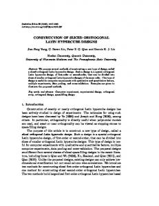
The results from the binGA, the permGA, the corresponding RLH DoE, and two existing DoE formulations from Refs. 5 and 16 are given in Table 3. Also shown in Table 3 is the number of function evaluations required to reach the binGA and permGA solutions. Comparisons with two previous DoE techniques from Ref. 5 and Ref. 16 show that the DoE formulated using the binGA and permGA methods perform better because they achieve solutions lower potential energies. It can be seen that the permGA solutions result in improvements over the binGA solutions and require on average 46-times fewer function evaluations to reach. It can be concluded, that the two methods work and that the permGA method is an effective tool for developing OLH DoE. The DoE for problem 3 (2 design variables and 120 points) is shown in Fig. 4. Fig. 4(a) shows the RLH DoE generated using Ref. 16, (b) shows the OLH DoE formulated using the binGA and (c) shows the OLH DoE formulated using the permGA. It would be expected from the results given in Table 4, that RLH has the worst uniformity and permGA has the best uniformity. A qualitative inspection of Fig. 4 confirms this. Design

Problem number Number of variables × Points 1 2 ×5

RLH from Ref. 2.7471 16

2 2 × 10

3 2 × 120

4 3 ×5

5 3 × 10

6 3 × 120

7 5 × 50

8 5 × 120

4.0772

10.4438

2.1068

2.3020

2.6404

0.8849

0.8903

−

−

−

0.7320

−

AELH –results from Ref. 5

−

2.1065

−

BinGA

1.2982 (60)

2.0662 (39,240)

5.7733 0.7267 (22,003,500) (5260)

1.0401 (165,980)

2.0541 (5,908,540)

0.7348 0.8003 (280,000,000) (59,802,200)

PermGA

1.2982 (50)

2. 0662 (1860)

5.5174 (130,570)

1.0242 (38,950)

1.9613 (1,996,920)

0.7270 (1,996,840)

0.7267 (1922)

0.7930 (1,998,540)

Table 3: Potential energy comparison of RLH designs from Ref. 16, AELH designs from Ref. 5, binGA designs and permGA designs, with the number of function evaluations required shown in brackets where appropriate

IV.

Conclusions

A method based on the application of a genetic algorithm to the formulation of the OLH DoE using the AudzeEglais objective function is proposed. Two formulations were considered, the first uses a binary encoded GA and the second uses a permutation encoded GA. The shortcomings of the former method are highlighted and the latter method was developed in response. It has been shown, that the formulation of OLHs is ideally suited to using GAs 6 American Institute of Aeronautics and Astronautics

(a) RLH (b) binGA (c) permGA Figure 4: Plan points for problem 3 (N=2 and P=120), generated using several methods since the problem uses discrete design variables. It can be seen, that a binary encoding, and the inherent need for a penalization method, can be used to solve the problems. But, it has also been shown that the use of a permutation encoding is better suited to the problem, because it is computationally more efficient; the permutation encoding requires fewer function evaluations and produces improved solutions. Further work is necessary to fully assess the quality of the results found using the permGA and the Audze-Eglais objective function. A comparison to the formulations with other objective functions, such as those discussed in Section II, can achieve this. Overall, it can be concluded, that the permGA method is an effective tool for developing OLH DoE.

Acknowledgements We gratefully acknowledge the financial support from EPSRC under the projects 'A Flexible Framework For Large Scale Optimization with Industrial Application' (Ref No. 00314975) and 'Computer Aided Optimisation of Extrusion Die Design' (EPSRC GR/M 95820). The third author would like to acknowledge financial support of the International Association for the promotion of cooperation with scientists from the New Independent States of the former Soviet Union (INTAS), project 600-2001.

References 1

Myers, R.H. and Montgomery, D.C. “Response surface methodology: Process and Product Optimization Using Designed Experiments”, John Wiley & Sons, New York, NY, 1976. 2 Mackay, M. D., Beckman, R. J., and Conover, W. J., “A comparison of three methods for selecting values of input variables in the analysis of output from a computer code”, Technometrics, Vol. 21, pp. 239-245, 1979. 3 Iman, R.L., and Conover, W.J., “Small sample sensitivity analysis techniques for computer models, with an application to risk assessment”, Communications in Statistics, Part A. Theory and Methods, 17:1749-1842, 1980. 4 Michalewicz, Z., “Genetic algorithms + data structures = evolution programs”, Springer-Verlag, 1992. 5 Bates, S. J., Sienz, J. and. Langley, D. S., “Formulation of the Audze–Eglais Uniform Latin Hypercube design of experiments”, J. Advances in Engineering Software, vol. 34/8 pp. 493 – 506, 2003. 6 Shewry, M., and Wynn, H., “Maximum entropy design”, J. Appl. Statist. 14 (2), pp. 165-170, 1987. 7 Sacks, J., Schiller, S.B., and Welch, W.J., “Designs for computer experiments” Technometrics 34, pp. 15-25, 1989. 8 Johnson, M., Moore, L., and Ylvisaker, D., “Minimax and maximin distance designs”, J. Statist. Plann. Inference 26, pp. 131-148, 1990. 9 Jin, R., Chen, W., and Sudjianto, A., "An Efficient Algorithm for Constructing Optimal Design of Computer Experiments" DETCDAC48760, 2003 ASME Design Automation Conference, Chicago, IL, September 2-6, 2003. 10 Audze, P., and Eglais, V., “New approach for planning out of experiments”, Problems of Dynamics and Strengths; 35:104-107. Zinatne Publishing House, 1977. 11 Merriam-Webster online dictionary. http://www.m-w.com 12 Bates, S.J. “Development of Robust Simulation, Design and Optimization Techniques for Engineering Applications”, PhD Thesis, University of Wales Swansea, 2003. 13 Oliver, I.M., Smith, D.J., and Holland, J.R.C., “A study of permutation crossover operators on the travelling salesman problem”, Proc. 2nd Int. Conf. on Genetic Algorithms, Massachusetts Institute of Technology, Cambridge, MA, pp411-423, 1987. 14 Goldberg, D.E., and Lingle, R., “Alleles, Loci, and the TSP”, proc. 1st Int. conf. on Genetic Algorithms, Hillsdale, NJ, pp154-159, 1985. 15 Davis, L., “Applying adaptive algorithms to epistatic domains”, proc. Int. Joint conf. on Artificial Intelligence, pp162-164, 1985. 16 Latin Hypercube sampling tool from web-page http://www.mathepi.com/epitools/lhs/nrpage.html , 2001.

7 American Institute of Aeronautics and Astronautics