Efficiency of a Boris-like integration scheme with ... - Semantic Scholar

PHYSICAL REVIEW SPECIAL TOPICS - ACCELERATORS AND BEAMS, VOLUME 5, 094001 (2002)

Efficiency of a Boris-like integration scheme with spatial stepping P. H. Stoltz* and J. R. Cary Tech-X Corporation, 5541 Central Avenue, Suite 135, Boulder, Colorado 80301

G. Penn and J. Wurtele Department of Physics, University of California, Berkeley, California 94720 (Received 4 June 2002; published 6 September 2002) A modified Boris-like integration, in which the spatial coordinate is the independent variable, is derived. This spatial-Boris integration method is useful for beam simulations, in which the independent variable is often the distance along the beam. The new integration method is second order accurate, requires only one force calculation per particle per step, and preserves conserved quantities more accurately over long distances than a Runge-Kutta integration scheme. Results from the spatial-Boris integration method and a Runge-Kutta scheme are compared for two simulations: (i) a particle in a uniform solenoid field and (ii) a particle in a sinusoidally varying solenoid field. In the uniform solenoid case, the spatial-Boris scheme is shown to perfectly conserve for any step size quantities such as the gyroradius and the perpendicular momentum. The Runge-Kutta integrator produces damping in these conserved quantities. In the sinusoidally varying case, the conserved quantity of canonical angular momentum is used to measure the accuracy of the two schemes. For the sinusoidally varying field simulations, error analysis is used to determine the integration distance beyond which the spatial-Boris integration method is more efficient than a fourth-order Runge-Kutta scheme. For beam physics applications where statistical quantities such as beam emittance are important, these results imply the spatial-Boris scheme is 3 times more efficient. DOI: 10.1103/PhysRevSTAB.5.094001

I. INTRODUCTION The Boris integration scheme [1,2] is popular in electromagnetic particle-in-cell simulations because it requires only one force evaluation per step while being second order accurate. In contrast, the commonly used fourth-order Runge-Kutta (RK) scheme [3] requires four force evaluations per step. The Boris integration scheme alternates position advance with acceleration, and the acceleration is broken into a half step of electric acceleration, followed by a rotation due to the magnetic field, followed by a half step of electric acceleration. The Boris integration scheme additionally better preserves conserved quantities, and it is stable for cyclotron integration for arbitrary step size. Consequently, the Boris scheme can be more efficient for many applications. Beam simulations are often carried out with the distance along the beam line being the independent integration variable, because that makes matching to spatial structures (such as the ends of magnets) easier. For such simulations one would like to have an integration method with the good properties of the Boris integrator. One cannot use the Boris integrator directly, as its derivation depends on one having a temporal integration. However, we show that one can derive a Boris-like integration scheme for the

*Email address: [email protected]

1098-4402兾02兾5(9)兾094001(9)$20.00

PACS numbers: 02.60.Cb, 02.70.Ns, 41.75.Ak, 52.59.Wd

case where one of the spatial coordinates is the independent variable. We compare the spatial-Boris scheme with a fourthorder RK scheme for two magnetic field configurations: (i) a uniform solenoid field and (ii) a sinusoidally varying solenoid field. In the uniform solenoid case, the spatialBoris scheme is shown to perfectly preserve for any step size conserved quantities such as the gyroradius and the perpendicular momentum. In contrast, the RK scheme produces an artificial damping of these quantities. We give a qualitative argument that for simulations in a uniform solenoid field, the spatial-Boris scheme should always be the more efficient scheme (where efficiency is defined by the number of force evaluations required). In the sinusoidally varying case, the conserved quantity of canonical angular momentum is used to measure the accuracy of the two schemes. The errors introduced by the spatial-Boris scheme produce an oscillation around the correct value, while the errors introduced by the RK scheme produce a secular change away from the correct value. Because of this, the spatial-Boris will be more accurate over a long enough distance. For the sinusoidally varying field, we compare error magnitudes to determine the integration distance beyond which the spatial-Boris integration method is more efficient than a fourth-order RK scheme. For typical beam physics applications, this error analysis shows that in a simulation of 103 lattice periods and 106 particles, the spatial-Boris scheme is 3 times more efficient. © 2002 The American Physical Society

094001-1

P. H. STOLTZ et al.

PRST-AB 5

This paper is organized as follows. In Sec. II, we derive the spatial-Boris scheme. In Sec. III, we compare the spatial-Boris scheme and a fourth-order RK scheme for simulations of particle motion in a uniform solenoid field. In Sec. IV, we compare the two schemes for simulations of particle motion in a sinusoidally varying solenoid field. Finally, in Sec. V, we discuss the implications for beam physics simulations, where we show the spatialBoris scheme may be 3 times more efficient for typical simulations. II. THEORY The motivation for how to modify the Boris scheme to use a spatial independent variable comes from relativity and Hamiltonian theory. Both of these subjects give formal methods for exchanging spatial and temporal variables. We begin by writing the momentum evolution equations, but substituting the energy evolution equation for the momentum component conjugate to the variable we want to become the independent variable (z in this paper): dpx 苷 q共Ex 1 yy Bz 2 yz By 兲 , (1) dt dpy 苷 q共Ey 1 yz Bx 2 yx Bz 兲 , dt

(2)

d共U兾c兲 苷 q共Ex yx 1 Ey yy 1 Ez yz 兲 , (3) dt where pz2 苷 共U兾c兲2 2 px2 2 py2 2 m2 c2 (MKS units). One exchanges z for t on the left-hand side by multiplying through by 1兾yz : µ ∂ y y Bz 1 dpx Ex dpx 苷 苷q (4) 1 2 By , dz yz dt yz yz µ ∂ Ey dpy 1 dpy y x Bz 苷 苷q (5) 2 1 Bx , dz yz dt yz yz µ ∂ y y Ey 1 dU兾c y x Ex Ez dU兾c 苷 苷q 1 1 . (6) dz yz dt yz c yz c c Exchanging yz for pz on the right-hand side, one can write this as a matrix equation, splitting into terms that involve pz and those that do not: dw 苷 Mw 1 b , (7) dz where 0 1 px (8) w 苷 @ py A , U兾c 1 0 0 Bz Ex 兾c q @ 2Bz 0 Ey 兾c A , M苷 (9) pz E 兾c E 兾c 0 x y and 0 1 2By (10) b 苷 q @ Bx A . Ez 兾c 094001-2

094001 (2002)

Only the matrix, M, involves pz . The equation for the evolution of the generalized particle position, s 苷 关x, y, ct兴, can be written ds w 苷 . dz pz

(11)

Equations (7) and (11) are the equations one needs to advance in the numerical integration scheme. The goal is to find a scheme that will advance these two sets of equations with second-order accuracy while requiring only one force evaluation per step. One can leapfrog [4] the advance of the generalized positions Eq. (11) with the generalized momenta Eq. (7). This means advancing the positions one-half a step, advancing the momenta a full step, and advancing the positions half a step. In this scheme, one assumes that the momenta are constant when advancing the positions and that the positions are constant when advancing the momenta. This will be at least second order accurate so long as each piece is at least second order accurate. The integration of the positions is exact assuming constant momenta, so one must only find a way to integrate the momentum equation to second order accuracy. As with the temporal Boris scheme, the approach here will be to further split the advance of Eq. (7) in a leapfrog way: (i) advance w first by only the vector term, b, for one-half a step, (ii) advance by only the matrix term, M, a full step, then (iii) advance by the vector b a final one-half step. Because the positions are assumed constant in the momentum advance, all the terms in b are constant, and so steps (i) and (iii) are exact. All that is left, then, is to show step (ii) can be done to second order accuracy. So long as the elements of M are all constant during this step, a space-centered advance (i.e., using the average of w on the right-hand side and solving the resulting implicit equation) is second order accurate. To show that M is constant, one needs to show that the coefficient pz is constant during step (ii). Because M involves only the field components Bz , Ex , and Ey that do not directly modify pz , one expects that pz will be constant. Formally, one can show that pz does not change magnitude when operated on by M by considering ∂ µ dpy dpz dpx 1 dU兾c 苷 2 px 2 py . (12) U兾c dz pz dz dz dz Using the equations of motion from Eq. (7) but including only the matrix term gives ∂∏ ∑ µ Ey py q Ex px dU兾c 苷 U兾c 1 , U兾c dz pz c c ∂∏ ∑ µ q dpx Ex U 苷 px Bz py 1 2 , (13) px dz pz c ∂∏ ∑ µ dpy Ey U q py 苷 py 2Bz px 1 2 . dz pz c

094001-2

EFFICIENCY OF A BORIS-LIKE INTEGRATION …

PRST-AB 5

Substituting into Eq. (12) yields (for the matrix term alone): dpz 苷 0. dz

(14)

Thus all change in the magnitude of pz is due to the vector b. This means that for a step involving only the matrix term, the elements of the matrix are constant, and a spacecentered advance will be second order accurate. Using the space-centered advance scheme for step (ii) means that one must solve an implicit equation. One uses the average w on the right-hand side of the equation: ∂ µ 1 w 1 w2 1 2 w 2w 苷M Dz , (15) 2

R苷

Dz 2 M 2 2 lˆ 2 Dz 2 4

DzM 1

11 0 b1 B B d E x Ey 苷 aB B 21 1 2 B2z c2 @ Ex d Ey Bz c 2 2 Bz c

To calculate 共I 2 MDz兾2兲 , one needs the eigenvalues of M. The eigenvalues of M are qq 2 l 苷 0, 6i (17) Bz 2 Ex2 2 Ey2 苷 0, 6i lˆ . pz

One can then write the matrix from Eq. (16) in a basisindependent way: µ ∂ µ ∂ Dz 21 Dz I 2M I 1M 2 2 苷I 1

Dz 2 兾2 Dz M 1 M2. 1 1 lˆ 2 Dz 2 兾4 1 1 lˆ 2 Dz 2 兾4 (19)

So one can advance from w 2 to w 1 using Eq. (16) rewritten as w1 苷 w2 1 1

Dz Mw 2 1 1 lˆ 2 Dz 2 兾4

Dz 2 兾2 M 2w2. 1 1 lˆ 2 Dz 2 兾4

The full operator for advancing w out as

2

to w

w 1 苷 w 2 1 Rw 2 , where from Eq. (21): 094001-3

1

(20)

can be written (21)

b2 Ey Bz c

Ex Bz c Ey Bz c

d Ex 2 Bz c

1

d 2 d 2

1 2 b3

Ey Bz c Ex Bz c

1 C C C C, A

where d

a苷

2共 2 兲 d

1 1 共 2 兲2 共1 2

Ex2 1Ey2 B2z c2 兲

,

(23)

and d苷

qBz Dz 苷 kDz , pz

(24)

b1 苷

µ ∂ d Ex2 2 1 , 2 Bz2 c2

(25)

b2 苷

µ 2 ∂ d Ey 2 1 , 2 Bz2 c2

(26)

21

In the corresponding basis of eigenvectors, this leads to 0 1 0 0 ∂ µ B1 C ˆ B C 11i lDz兾2 Dz 21 B C 0 0 2 2 苷B I 2M 11lˆ Dz 兾4 C . (18) @ A 2 ˆ 12i lDz兾2 0 0 2 2 ˆ 11l Dz 兾4

d Ex Ey 2 Bz2 c2

11

(22)

2

where w is the vector before the matrix operation, and w 1 is the vector after. Solving for w 1 gives ∂ µ ∂ µ Dz 2 Dz 21 1 w . w 苷 I 2M I 1M (16) 2 2

094001 (2002)

µ ∂ Ey2 d Ex2 1 2 2 . b3 苷 2 B2z c2 Bz c

(27)

The quantity k 苷 qBz 兾pz defined in Eq. (24) is related to the distance, Zg 苷 2p兾k, over which a particle would complete an oscillation in a uniform field of strength Bz . The distance Zg is called the gyroperiod. We leave Eqs. (22)–(27) expressed in terms of d兾2 for reasons regarding the gyroperiod discussed below. To summarize, the final steps for the spatial-Boris push to move from position z n to z n11 are as follows: (1) Push the generalized positions one-half step (Dz兾2兲 using the velocities at z n . (2) Evaluate the fields at this midpoint time and position. (3) Push the generalized momenta vector, w, from w n to an intermediate state w 2 with a half step using only the vector b: w2 苷 wn 1

Dz b. 2

(28)

(4) Evaluate pz at this point, plug into the matrix R, and advance w 2 to w 1 with a full spatial step of the matrix part of Eq. (7): w 1 苷 w 2 1 Rw 2 .

(29)

(5) Advance w 1 to the final state w n11 with a half step using only the vector b: w n11 苷 w 1 1

Dz b. 2

(30)

094001-3

P. H. STOLTZ et al.

PRST-AB 5

(6) Push the generalized positions one-half step using the velocities at z n11 . The above steps require only one evaluation of the fields. One can combine steps (1) and (6) for efficiency, but the positions are then known one-half step off from the momenta. By keeping steps (1) and (6) separate, one knows the generalized positions and momenta at the same spatial location at the end of a step. III. SIMULATIONS IN A UNIFORM SOLENOID FIELD The RK scheme is known to produce artificial damping (or growth) of conserved quantities (see Fig. 3 of Ref. [5]). Because the spatial-Boris scheme is a leapfroglike scheme, we expect it to have improved conservation properties in the same way as symplectic integrators [6]. As a first test of this, we chose the problem of motion of a particle in a uniform solenoid field. For this problem, the gyroradius and perpendicular momentum are conserved quantities. The gyroradius is rg 苷

yp 21 k , yz

where yp is defined by q pp , yp 苷 yx2 1 yy2 苷 gm

(31)

(32)

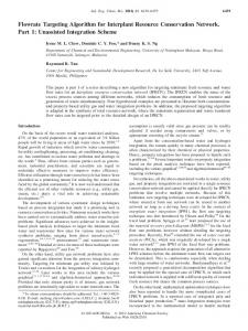
and pp is the perpendicular momentum. Figure 1 shows the radius as a function of distance for various step sizes for simulations using the RK scheme. In

FIG. 1. The gyroradius (normalized to its initial value) as a function of distance (normalized to the gyroperiod) calculated using the fourth-order Runge-Kutta integration scheme. Plots are shown for step sizes of 5, 7.5, 10, and 20 steps per gyroperiod. The curves for perpendicular momentum as a function of distance are similar to these.

094001-4

094001 (2002)

this figure, the gyroradius is normalized to its initial value and the distance of integration to the gyroperiod. This figure shows that the RK scheme produces artificial decay of the gyroradius, as expected from the results of Ref. [5]. The RK scheme also produces a decay in the perpendicular momentum. The curves of perpendicular momentum as a function of distance for the various step sizes are similar to those for the gyroradius, so we do not show them here. Figure 2 shows on a log-log plot the fractional error versus step size after one gyroperiod. The error scales as Dz 5 兾Zg5 . For a fourth-order integrator, one might expect the error for a fixed integration distance to scale as Dz 4 . This is because one might expect the error in a single step would go as estep ⬃ Dz 5 , and for a fixed distance of integration, the number of steps goes as N ⬃ Dz 21 . This implies the error would scale as e 苷 Nestep ⬃ Dz 4 . However, the coefficients for a single step of the RK scheme produce a coincidental cancellation of the fifth-order error in the calculation of the radius (see Appendix A). So, the error in calculation of the radius in a single step in fact goes as estep ⬃ Dz 6 , and so the total error goes as e 苷 Nestep ⬃ Dz 5 , as shown in Fig. 2. In contrast, for simulations using the spatial-Boris scheme, the gyroradius and perpendicular momentum are perfectly conserved for any step size. The full calculation of these quantities for a single step of the spatial-Boris integrator is shown in Appendix B. To demonstrate this conservation, Fig. 3 shows the radius as a function of distance for various step sizes for simulations using the spatial-Boris scheme. Figure 3 also shows the perpendicular momentum as a function of distance using the spatial-Boris integration scheme. These plots are put on

FIG. 2. The fractional error in the gyroradius after one gyroperiod as a function of steps per period using the Runge-Kutta scheme. The slope of the line is consistent with the error in the radius in a single step of the Runge-Kutta being sixth order.

094001-4

PRST-AB 5

EFFICIENCY OF A BORIS-LIKE INTEGRATION …

FIG. 3. The gyroradius and perpendicular momentum (normalized to their initial values) as a function of distance (normalized to the gyroperiod) calculated using the spatial-Boris scheme. These are plotted for a step size of five steps per gyroperiod. These quantities are perfectly conserved for any step size using the spatial-Boris scheme.

the same vertical scale as Fig. 1 for comparison, however the integration distance is many hundreds of times farther for the spatial-Boris simulations to demonstrate the conservation. The perfect conservation of rg and pp is not shown definitively by Fig. 3, but a detailed analysis does show the errors in rg and pp are zero to within the double-precision accuracy of the data analysis tool we used. Furthermore, we show rg and pp for a step size of five steps per period in Fig. 3, as this was the largest step size used in the Runge-Kutta analysis, and therefore 094001-5

094001 (2002)

should be a worst case. The perfect conservation does hold for all step sizes however. While the spatial-Boris scheme is good at preserving conserved quantities, it is still only a second-order integration scheme and does produce errors. In this case, the scheme introduces phase error. The phase for this case is defined as y tan共u兲 苷 , (33) x where u is the phase. One can show the error in phase introduced by the spatial-Boris scheme by considering the special case of initial conditions x 苷 x0 , y 苷 0, px 苷 0, and py 苷 2kx0 . For a single step, the phase should be u 苷 2p共Dz兾Zg 兲 苷 kDz, which gives to third order (using the notation d 苷 kDz): µ ∂ d3 tan共u兲 苷 tan共d兲 艐 2 d 1 . (34) 3 The minus sign is due to the clockwise rotation. However, following the evolution (see Appendix B) through one step of the spatial-Boris scheme gives ∂ µ d 22共 2 兲 y d3 苷 . (35) 艐2 d1 d x 4 1 2 共 2 兲2 The spatial-Boris scheme produces a phase slightly smaller than the true phase, meaning the calculated rotation is too slow. The phase error due to the spatial-Boris scheme is third order in Dz, as expected for a second-order integrator. Integrated over an entire period, the spatial-Boris scheme introduces an error in the gyroperiod that is second order in Dz. However, Boris [1] points out that replacing d兾2 with tan共d兾2兲 in Eqs. (22)–(27) will correct the phase error to all orders. The motivation for this modification is seen in Eq. (35), where making the replacement yields the trigonometric identity d 22 tan共 2 兲 y 苷 (36) d 苷 tan共d兲 . x 1 2 tan2 共 2 兲 Boris refers to this as the tan共a兲兾a modification. Because to first order tan共d兾2兲 苷 d兾2, and the next term is third order in d兾2, the modification to the step size is third order and so does not affect the order of accuracy of the individual positions or momenta. For simulations in a uniform magnetic field, where gyromotion is the dominant motion, the tan共a兲兾a modification is clearly an improvement over the unmodified scheme. For simulations in spatially varying fields, this modification changes the spatial dependence of the coefficients in Eqs. (22)–(27) and changes the effective step size. Dynamically changing the step size in a leapfrog scheme has been shown [7] to introduce a secular error in conserved quantities, so applying the tan共a兲兾a modification to spatially varying fields must be done with care. The conservation properties of the spatial-Boris scheme make it almost certainly the more efficient integrator for 094001-5

PRST-AB 5

P. H. STOLTZ et al.

this problem (where efficiency is measured in terms of the force evaluations required). The conservation of the topology for any step size means that typically one would choose the step size based on other considerations (perhaps resolving some other feature of the problem). For instance, a modest restriction on step size of 20 steps per period with the spatial-Boris scheme means that scheme would require 20 force evaluations per period. Because the RK scheme requires four force evaluations per step, to be as efficient as the spatial-Boris scheme at 20 steps per period, the RK scheme would have to use only five steps per period. Figure 1 shows that for five steps per period, the RK scheme can introduce errors of over 10% after only a few periods. While this argument is only qualitative and does not account for the phase errors introduced by the spatial-Boris scheme, for most problems involving a uniform solenoid field, the advantages of the spatial-Boris scheme will outweigh any disadvantages. IV. SIMULATIONS IN A SINUSOIDALLY VARYING SOLENOID FIELD As a second test of the different integration schemes, we looked at simulations of particle motion in a sinusoidally varying solenoid field. The z component of the magnetic field used in these simulations is shown in Fig. 4. The radial component of the magnetic field is chosen to satisfy = ? B 苷 0. The distances for this problem are scaled to the spatial oscillation period of the magnetic field, which we call the lattice period and denote by ZL . In this case, the gyroradius and perpendicular momentum are not conserved quantities, but the canonical angular

FIG. 4. Bz (normalized to its peak value) as a function of distance (normalized to the lattice period) from simulations with a sinusoidally varying magnetic field. The magnitude of Br is calculated to satisfy =B 苷 0.

094001-6

094001 (2002)

momentum is conserved. The canonical angular momentum is Lc 苷 r共p 1 qA兲 ,

(37)

where A is the vector potential, and we consider only the component of the canonical angular momentum parallel to B. Figure 5 shows the longitudinal part of the canonical angular momentum (normalized to its initial value) as a function of distance (normalized to the lattice period) for both schemes. The solid line shows the results using the spatial-Boris scheme, and the dashed line shows the results using the RK scheme. Both plots show results from simulations with a step size of ten steps per lattice period. This figure exhibits the behavior seen previously in comparisons of RK to other integration schemes (see Figs. 3 and 4 of Ref. [5]). The RK scheme introduces a secular error in the longitudinal part of Lc , while the spatial-Boris scheme introduces an oscillatory error. This implies that for long enough integration distances, the spatial-Boris scheme will be more accurate. Figure 6 shows the fractional error as a function of step size for both schemes. The error due to the RK scheme (calculated after 100 lattice periods and shown as triangles) again scales as Dz 5 , as it did for the case of the gyroradius in a uniform field. The error due to the spatial-Boris scheme (shown as squares) is independent of the final distance and is measured as the amplitude of the oscillations seen in Fig. 5. The error for the spatial-Boris scheme scales as Dz 2 , as expected for a second-order integration scheme (the error in a single step is of order Dz 3 , but the accumulated error over many steps

FIG. 5. The longitudinal part of the canonical angular momentum (normalized to its initial value) as a function of distance (normalized to the lattice period) for a step size of ten steps per lattice period. The dashed line shows results using the Runge-Kutta scheme, and the solid line shows results using the spatial-Boris scheme. The Runge-Kutta scheme produces a secular drift, while the spatial-Boris scheme produces oscillation.

094001-6

EFFICIENCY OF A BORIS-LIKE INTEGRATION …

PRST-AB 5

FIG. 6. Fractional error in the longitudinal canonical angular momentum as a function of steps per lattice period for the Runge-Kutta and spatial-Boris schemes. The error from the Runge-Kutta scheme is shown by triangles, and the error from the spatial-Boris scheme is shown by squares. The error in the RK scheme is measured after 100 lattice periods. The error in the spatial-Boris scheme is independent of the final integration distance. 2

scales as Dz ). One might expect the canonical angular momentum calculated using the spatial-Boris scheme to oscillate about the initial value, thereby conserving canonical angular momentum on average. However for symplectic integrators, it is known that the finite size of the integration step shifts the invariants [8], and these shifted invariants are not guaranteed to be symmetric about the original invariants. Unlike the uniform solenoid field, for the sinusoidally varying solenoid field both integrators are introducing errors into the conserved quantities. The RK errors are secular, while the spatial-Boris errors are oscillatory, and consequently one expects the spatial-Boris scheme to be more efficient for long integration distances. However, the RK scheme is a more accurate (fourth-order) scheme than the spatial-Boris (second-order), and consequently one expects the RK scheme to be more efficient for short integration distances. Given a distance of integration, one can calculate the accuracy level at which the spatial-Boris and RK integrators require the same number of force evaluations, NF , and therefore are equally efficient. We call this accuracy level the crossover error. The error as a function of the final distance for the RK scheme is eRK 苷 b

5

Zf Dz Zf 苷 b0 5 , ZL ZL ZL

(38)

where b0 is a constant and Zf is the final distance. The error due to the spatial-Boris scheme is given by 094001-7

094001 (2002)

FIG. 7. The crossover error (the fractional error level at which the Runge-Kutta and spatial-Boris schemes use the same number of force calculations) as a function of the integration distance in lattice periods for a sinusoidally varying solenoid field. For points to the left of the line, the Runge-Kutta scheme uses fewer force calculations. For points to the right of the line, the spatialBoris scheme uses fewer force calculations.

Dz 2 , (39) ZL2 where eB0 is also a constant. From Fig. 6, we know b0 艐 80.0 and eB0 艐 3.0. The number of steps required for a given step size and integration distance is N 苷 Zf 兾Dz. We denote the number of steps for the spatial-Boris scheme as NB 苷 NF and for the RK scheme as NRK 苷 NF 兾4. Setting Eq. (38) equal to Eq. (39) gives Zf5 共Zf 兾NB 兲2 苷 b Zf 兾ZL . (40) e 苷 eB0 0 5 ZL2 NRK ZL5 Substituting in and solving for NF and plugging back into either Eq. (38) or Eq. (39) gives the crossover error, eC , in terms of Zf 兾ZL : µ ∂22兾3 5兾3 Zf eB0 eC 苷 . (41) 2兾3 ZL 410兾3 b0 eB 苷 eB0

Figure 7 shows eC as a function of Zf 兾ZL for b0 苷 80.0 and eB0 苷 3.0. For points to the left of the line, the RungeKutta scheme uses fewer force calculations. For points to the right of the line, the spatial-Boris scheme uses fewer force calculations. V. IMPLICATIONS FOR BEAM PHYSICS SIMULATIONS In this section, we discuss the implications of the efficiency of the spatial-Boris scheme for typical beam physics simulations. We show that for calculations where statistical errors are dominant (like the calculation of beam 094001-7

P. H. STOLTZ et al.

PRST-AB 5

emittance), the spatial-Boris scheme is more efficient over distances typical of beam physics simulations. We estimate that for simulations using approximately 106 particles and going roughly 103 gyroperiods, the spatial-Boris scheme is approximately 3 times more efficient. A common calculation in beam physics is the beam emittance. The emittance for the x direction, for instance, is defined as ex2 苷 具x 2 典 具px2 典 2 具xpx 典2 .

(42)

This is a statistical quantity and so is subject to statistical noise because there are usually fewer computational particles than beam particles. For instance, if a simulation 6 uses p 10 particles, the statistical errors will be on the order of 1兾106 苷 1023 . Accelerators are typically a few hundred meters long, with lattice periods on the order of a fraction of a meter, so Zf 兾ZL 艐 103 . Figure 7 shows that for Zf 兾ZL 艐 103 the spatial-Boris scheme will be more efficient for e 艐 1023 . In fact, using Eq. (39) and e 艐 1023 gives a step size for the spatial-Boris scheme of µ ∂ Dz 艐 0.02 . (43) ZL B The spatial-Boris scheme uses one force evaluation per step, and so a simulation of Zf 兾ZL 艐 103 would require 5 3 104 force evaluations. By comparison, Eq. (38) gives µ ∂ Dz 艐 0.025 . (44) ZL RK The RK scheme uses four force evaluations per period, so a simulation of Zf 兾ZL 艐 103 would require approximately 1.6 3 105 force evaluations. For these parameters, the spatial-Boris scheme is roughly 3 times more efficient. In other words, if the computation time in the simulation is dominated by force evaluations (as it will be for many codes), a simulation using the spatial-Boris scheme should run 3 times faster than a simulation using the RK scheme. VI. CONCLUSION We have developed a modified Boris-like integration, in which a spatial coordinate is the independent variable. This spatial-Boris integration method is useful for beam simulations, in which the independent variable is often the distance along the beam. The new integration method is second order accurate, requires only one force calculation per particle per step, and preserves conserved quantities more accurately over long distances than a Runge-Kutta integration scheme. We compared results from the spatialBoris integration method and a Runge-Kutta scheme for two simulations: a particle in a uniform solenoid field and a particle in a sinusoidally varying solenoid field. In the uniform solenoid case, the spatial-Boris scheme conserves perfectly for any step size quantities such as the gyroradius 094001-8

094001 (2002)

and the perpendicular momentum. The Runge-Kutta integrator produces damping in these conserved quantities. For the sinusoidally varying field simulations, error analysis is used to determine the integration distance beyond which the spatial-Boris integration method is more efficient than a fourth-order Runge-Kutta scheme. For beam physics applications where statistical quantities such as beam emittance are important, these results imply the spatial-Boris scheme is 3 times more efficient. A possible application of this work is to provide an alternate algorithm for self-consistent simulations. Lidia, for example, has recently developed [9] a self-consistent klystron simulation code that calculates part of the propagation using approximate maps obtained by integration of trajectories. The spatial-Boris integrator might be used for obtaining these maps. There is no guarantee that the map obtained by spatial-Boris integration is symplectic, but it does have many of the good qualities of symplectic integrators, such as no secular change of conserved quantities. ACKNOWLEDGMENTS The authors thank D. Bruhwiler, W. Fawley, and R. Fernow for many suggestions regarding this work. This work was funded in part by the Department of Energy Division of High-Energy Physics and in part by Tech-X Corporation. APPENDIX A: CALCULATION OF THE GYRORADIUS IN A UNIFORM SOLENOID WITH THE RUNGE-KUTTA INTEGRATION SCHEME In this appendix, we show that calculating the gyroradius with a fourth-order RK scheme for a uniform solenoid field gives a fortuitous cancellation of the expected fifth-order error. This explains the scaling of the error seen in Fig. 2. The exact expression for the gyroradius in a uniform field is x共z兲 苷 x0 cos共kz兲 1 y0 sin共kz兲 ,

(A1)

y共z兲 苷 y0 cos共kz兲 2 x0 sin共kz兲 ,

(A2)

where k 苷 qB兾pz . In a single step of dimensionless size d 苷 kDz, the RK scheme gives the same result as Taylor expanding the exact expression to fourth order: ∂ ∂ µ µ d4 d2 d3 xn11 苷 xn 1 2 1 1 yn d 2 , (A3) 2 24 6 ∂ ∂ µ µ d4 d2 d3 yn11 苷 yn 1 2 1 2 xn d 2 . 2 24 6

(A4)

To calculate the radius, we need to square x and y. Keeping terms to sixth order, squaring the above gives 094001-8

EFFICIENCY OF A BORIS-LIKE INTEGRATION …

PRST-AB 5

pxn11 苷 pxn 1

2 xn11 苷 xn2 1 d共2xn yn 兲 1 d 2 共yn2 2 xn2 兲

∂ 4 1 1 d 2 xn yn 1 d 4 共xn2 2 yn2 兲 3 3 µ ∂ µ ∂ 1 2 5 1 6 1 2 xn yn 1 d y 2 x , 1d 4 36 n 24 n (A5) 3

µ

2 苷 yn2 1 d共22xn yn 兲 1 d 2 共xn2 2 yn2 兲 yn11 µ ∂ 1 3 4 xn yn 1 d 4 共yn2 2 xn2 兲 1d 3 3 ∂ µ ∂ µ 1 2 1 2 1 xn 2 yn . 1 d 5 2 xn yn 1 d 6 4 36 24 (A6)

The odd terms in these expressions are of opposite sign, and so when one calculates the radius, r 2 苷 x 2 1 y 2 , only even terms will survive. Further, the second-order and fourth-order terms cancel as expected. Thus, the change in radius squared from n to n 1 1 is

d6 2 共x 1 yn2 兲 . 72 n

2b 共2bpyn 2 pxn 兲 . 1 1 1 b2

(B2)

According to the spatial-Boris scheme, the positions get a half-step kick with the momenta at n and a half-step kick with the momenta at n 1 1. This gives µ ∂ pyn pxn pxn Dzb n11 n 苷x 1 Dz 1 1 2b , x pz 1 1 b2 pz pz µ ∂ pyn pyn pxn Dzb Dz 1 2 2b . y n11 苷 y n 1 pz 1 1 b2 pz pz (B3) By using the initial conditions pxn 苷 kyn pz and pyn 苷 2kxn pz and working through the algebra, one gets 共pxn11 兲2 1 共pyn11 兲2 苷 共pxn 兲2 1 共pyn 兲2 , 共x n11 兲2 1 共y n11 兲2 苷 共x n 兲2 1 共y n 兲2 .

(B4)

(A7)

Taking the square root to get from r 2 to r will not affect the order of the error. This shows the error in radius in one step of a fourth-order RK is sixth order. APPENDIX B: CALCULATION OF GYRORADIUS AND PERPENDICULAR MOMENTUM IN A UNIFORM SOLENOID WITH THE SPATIAL-BORIS INTEGRATION SCHEME In this appendix, we show that calculating the gyroradius and perpendicular momentum with the spatial-Boris scheme in a uniform solenoid field yields zero error. For the case where Bz is the only field component, the matrix R in Eq. (22) is 0 1 1 0 2b @ 2b (B1) R苷 21 2b 0 A , 1 1 b2 0 0 0 where b 苷 kDz兾2. This means after one step from n to n 1 1, the momenta become

094001-9

苷

pyn

2b 共2bpxn 1 pyn 兲 , 1 1 b2

Thus the perpendicular momentum and gyroradius are conserved exactly by the spatial-Boris scheme.

2 2 2 rn11 2 rn2 苷 共xn11 1 yn11 兲 2 共xn2 1 yn2 兲

苷2

pyn11

094001 (2002)

[1] J. Boris, in Proceedings of the Fourth Conference on Numerical Simulation of Plasmas, edited by J. P. Boris and R. A. Shanny (Naval Research Laboratory, Washington, D.C., 1970), pp. 3– 67. [2] C. Birdsall and A. Langdon, Plasma Physics Via Computer Simulation (McGraw-Hill, Inc., New York, 1985), pp. 356–359. [3] W. H. Press, S. A. Teukolsky, W. T. Vetterling, and B. P. Flannery, Numerical Recipes in C: The Art of Scientific Computing (Cambridge University Press, Cambridge, 1993), pp. 710– 714. [4] S. Godunov, Math. USSR-Sb 47, 271 (1959). [5] A. Dullweber, B. Leimkuhler, and R. McLachlan, J. Chem. Phys. 15, 5840 (1997). [6] E. Forest and R. Ruth, Physica (Amsterdam) 43D, 105 (1990). [7] P. Hut, J. Makino, and S. McMillan, Astrophys. J. 443, L93 (1995). [8] A. Lichtenberg and M. Lieberman, Regular and Chaotic Dynamics (Springer-Verlag, New York, 1992), 2nd ed., pp. 169 –174. [9] S. M. Lidia, Phys. Rev. ST Accel. Beams 4, 041001 (2001).

094001-9