Efficient Algorithms for Performance Management of Computing Systems∗ Jia Bai
Institute for Software Integrated Systems Vanderbilt University Nashville, Tennessee 37235
[email protected]
ABSTRACT This paper addresses the problem of managing computing systems using an integration of model-based control techniques and efficient AI search strategies. The control approach uses the system model to forecast all future system behavior up to a certain horizon and then searches for the best path for the system based on a given utility function. In practical computing systems, however, the large number of control (tuning) options directly affects the computational overhead of the control module which executes in the background at run-time, and ultimately slows down the overall system. To handle this problem, several search algorithms are introduced to improve the controller’s performance. A case study of an online processor power management is used to demonstrate the effectiveness of the new search techniques for the model-based control approach.
Keywords optimization, search algorithm, predictive control, modelintegrated computing
1.
INTRODUCTION
Our society has become increasingly dependent on services provided by distributed computing systems. Consequently, there has been an exponential increase in the complexity of computer systems in recent times. These systems often host information technology applications vital to transportation, online banking and shopping, military command and control, among others. And they need to satisfy stringent performance requirements, such as service delay bounded by a relatively small constant. Moreover, they operate in highly dynamic environments, where the workload to be processed may be time varying and hardware or software components may fail or degrade during system operations. In order to achieve the performance requirements while operating in such dynamic environments, numerous performance-related ∗This work was supported in part through a grant from the NSF SOD program, contact number: CNS-0804230
Sherif Abdelwahed
Department of ECE Mississippi State University Mississippi State, Mississippi 39762
[email protected]
parameters must be continuously monitored, and if needed, optimized to respond rapidly to time-varying operating conditions. As they grow in scale and complexity, the conventional, manual management of these systems becomes more and more difficult, time-consuming, and error-prone. Accordingly, there is an increasing need for these systems to possess autonomic managing capillarities, thus, minimizing human intervention. With autonomic managing facilities, the systems will receive high-level objectives from human administrators [16] and maintain the specified requirements by adaptively tuning key operating parameters [10]. Control-theoretic strategies have been recently applied to the design and verification of various adaptive performance management schemes in computation systems. This approach offers some important advantages over rule-based policies for performance management in that a generic control framework can address a variety of problems, such as power management, resource allocation and provisioning, by using the same basic control concepts. If system dynamics are precisely modeled and the changing environmental parameters are accurately estimated, the appropriate runtime control algorithms can be effectively developed to realize system self-regulation and achieve desired objectives. Moreover, the feasibility or stability of the proposed control scheme with respect to the performance metrics can be verified prior to actual deployment. Examples of controltheoretic resource management strategies include task scheduling [18, 23], QoS guarantees in web servers [17], resource allocation control [11, 21] , network flow control [15], and power management [4]. In earlier work, a generic model-based control has been designed [1, 13, 14] to address self-managing problems in computing systems. A switching hybrid-system model [2] is adopted to capture the dynamics of systems having a finite control-input set. Using this system model, a limited lookahead control (LLC) technique is developed where control actions are obtained by optimizing system behavior, as forecast by a mathematical model, for the specified performance criteria over a limited look-ahead prediction horizon. Both the control objectives and operating constraints are represented explicitly in the optimization problem and solved for each time instant. The optimization problem is to minimize a multi-variable system utility function specifying the trade-offs between achieving the desired requirements and
the corresponding cost incurred in terms of resource usage. For example, a controller may be required to meet a certain response time for a time-varying workload while minimizing system power consumption. This method can be applied to a variety of performance management problems, from systems with simple dynamics to more complex systems exhibiting non-linear behavior or ones with long delay or dead times. This method can also accommodate changes to the behavioral model itself caused by resource failures and/or parameter changes in time-varying systems. In this paper, we address the complexity problem of the LLC algorithm, by considering several efficient search methods that can significantly reduce the size of the underlying search space. The implemented search algorithms are shown to improve the controller performance by reducing its overhead while maintaining the system at or close to the optimal point. The new search algorithms are demonstrated on a case study of a processor capable of dynamic voltage scaling (DVS) where operating frequencies can be chosen from a finite set. The management problem is to maximize the processor utilization, which is a trade-off between processing speed and power consumption, under a time-varying workload. The simulation results of the different searches are compared and evaluated. The rest of the paper is organized as follows. Section 2 reviews the LLC concepts. Section 3 presents in detail different search approaches. Section 4 discusses the implementation of a DVS-capable processor case study and provides test results of performances. We conclude the paper in Section 5.
2.
Figure 1: The limited lookahead control approach Table 1: The LLC Algorithm 1 2 3 4 5 6 7 8 9 10 11 12 13 14 15 16 17
OLC(x(k)) /* x(k) := current state measurement */ sk := x(k); Cost(x(k)) = 0 for all k within prediction horizon of depth N do Forecast environment parameters for time k + 1 sk+1 := ∅ for all x ∈ sk do for all u ∈ U do x ˆ = f (x, u, w) /* Estimate state at time k + 1 */ Cost(ˆ x) = Cost(x) + J(ˆ x) sk+1 := sk+1 ∪ {ˆ x} end for end for k := k + 1 end for Find xmin ∈ sN having minimum Cost(x) u∗ (k) := initial input leading from x(k) to xmin return u∗ (k)
ONLINE CONTROL CONCEPTS
In this section, we review the main concepts underlying the LLC approach. In this control approach, relevant parameters of the operating environment, such as workload arrival patterns, etc., are estimated and used by a system model to forecast future behavior over a look-ahead horizon. The controller optimizes the forecast behavior as per the specified performance requirements by selecting the best control inputs to apply to the system [1]. To apply mathematical techniques an abstract model of the underlying system is required. In the LLC approach, the dynamics of a computation system is captured using a switching hybrid system model – a special class of hybrid systems in which the control input set is finite. The following discrete-time equation describes the system dynamics: x(k + 1) = f (x(k), u(k), w(k)) Here, x(k) is the system state at time step k, while u(k) and w(k) denote the control inputs and environment parameters at time k, respectively. The system model f captures the relationship between the observed system parameters, particularly those relevant to the system specifications, and the control inputs that adjust these parameters. The control input set U is assumed finite. Many computing systems have a limited finite (quantized) set of control inputs and, therefore, their dynamics can be adequately captured using the above model. In general, computing systems are required to achieve specific performance objectives while satisfying certain operat-
ing constraints. A basic control action in such systems is set-point regulation where key operating parameters must be maintained at a specified level. The controller, therefore, aims to drive the system to within a close neighborhood of the desired operating state x∗ ∈ X in finite time and maintain the system there. As shown in Fig. 1, in the LLC approach, the next control action is selected based on a distance map defining how close the current state is to the desired set point. This map may be defined for each state x as D(x) = ||x − x∗ ||, where ||.|| is a proper norm. Table 1 shows the online control algorithm that aims to satisfy a given performance specification for the underlying system. At each time instant k, it accepts the current operating state x(k) and returns the best control input u∗ (k) to apply. Starting from this state, the controller constructs, in breadth-first fashion, a tree of all possible future states up to the specified prediction depth. Given the current state x(k), the relevant parameters of the operating environment are estimated, and the next set of reachable system states are generated by applying all valid control inputs from the set U . The cost function corresponding to each estimated state is then computed. Once the prediction horizon is fully explored, a unique sequence of reachable states x ˆ(k + 1), . . . , x ˆ(k + N ) that optimize the objective function is computed and the first input u∗ (k) along the path to x ˆ(k + N ) is applied to the system while the rest are discarded. The above control action is repeated each sampling step.
Table 2: Uniform-cost search algorithm for LLC 1 2 3 4 5 6 7 8 9 10 11 12 13 14 15 16 17
uni-OLC(x(k)) /* x(k) := current state measurement */ Q := x(k); Cost(x(k)) = 0; /*Q := priority queue */ while Q is not empty x := first element in Q, if depth(x) == N u∗ (k) := initial input leading from x(k) to x return u∗ (k) else for all u ∈ U do x ˆ = f (x, u, w) /* Estimate next state */ Cost(ˆ x) := Cost(x) + J(ˆ x) depth(ˆ x) := depth(x) + 1 Q := Q ∪ {ˆ x} end for sort Q according to Cost in an ascending order end if continue while
In a computation system where control inputs are chosen from discrete values, the LLC algorithm exhaustively evaluates all possible operating states within the prediction horizon to determine the best control input. Therefore, the size of the search tree grows exponentially with the number of inputs; if |U | denotes the size of the input set, and N the prediction depth, the number of explored states is given by PN j j=1 |U | . This is not a major concern for systems with few control options. However, with a large control-input set, the corresponding control overhead may be excessive for real-time performance.
3.
ENHANCED SEARCH TECHNIQUES
As shown in the previous section, the search process is responsible for the exponential growth of the control algorithm. To enhance the efficiency of the control algorithm, we apply several efficient search algorithms in the following sections that can be directly integrated with the LLC algorithm.
3.1
Uniform-cost Search
Uniform-cost search [20] is a tree search algorithm used for traversing or searching a weighted tree, tree structure, or graph. It begins at the root node, but instead of always expanding the shallowest node like breadth-first search, the uniform-cost search continues by visiting the next node with the least Cost - the accumulative path cost from the root to the current node. Nodes are visited in this manner until the goal state is reached. The uniform-cost search is complete and optimal if the cost of each step is greater than or equal to some small positive constant ². But when all path costs of the uniform-cost search are positive and identical, it changes back to breadth-first search.
panding nodes by adding all unexpanded neighboring nodes that are connected by directed paths to a priority queue. In the queue, each node is associated with its Cost, and the least-Cost node is given highest priority, so that the queue is sorted in an ascending order. The node at the head of the queue is subsequently popped and expanded, appending the next set of connected nodes with their Costs to the queue. The completeness and optimality of the uniform-cost search can be guaranteed by setting even-valued exponent terms in the utility function of the Cost(see Table 2) to make all the path costs positive. The utility function at time k can therefore take the form 2 J(k) = a1 y12 (k) + a2 y22 (k) + · · · + am ym (k)
with m parameters to optimize, yi (k), i ∈ m represents a performance related parameter at time k, and ai , i ∈ m is the user-specified weight denoting the relative importance of yi (k). In the control framework, usually different values are assigned to the components of the utility function, so the path costs will rarely be identical. The positive and nonidentical path costs provide promising supports for applying uniform-cost search in the control algorithm. But as uniform-cost search is guided by path costs rather than depths, sometimes its complexities cannot easily be characterized and its worst-case time and space complexities can be, in certain situations, greater than those of a breadth-first search.
3.2
A* Search
In the original control algorithm, we have only considered the path costs from the starting node to the current node, but not the possible costs from the current node to the goal node in the tree structure. A* search, one of the most widely-known form of best-first search, evaluates nodes by combining g(n), the cost to reach the node from the root, and h(n), the cost to get from the node to the goal: f (n) = g(n) + h(n) Then the algorithm complexity is determined by both g(n) and h(n). Note that uniform-cost search is a special case of the A* search when the heuristic h(n) is constant, so the A* search algorithm for LLC is similar to the LLC uniform-cost search in Table 2 except that the Cost is given by Cost(x(k) to node) + h(node) instead. A* is complete in the sense that it will always find a solution if there is one. However, its optimality depends on if h(n) is an admissible heuristic, or never overestimates the cost to reach the goal [20]. Formally, for all paths y, z where z is a successor of y, g(y) + h(y) ≤ g(z) + h(z)
The space complexity of the uniform-cost search is the number of nodes with Costs smaller than or equal to the cost of the optimal solution, plus the ones extended by those nodes. The time complexity is the time needed to process the nodes. Formally, if C ∗ is the cost of the optimal solution and it is assumed that every path cost is at least ², the algorithm’s ∗ complexity is O(b1+bC /²c ), instead of O(bd ) in breadth-first search [20].
A* is also optimally efficient for any admissible heuristic h; no algorithm employing the same heuristic will expand fewer nodes than A*, except when there are several partial solutions where h exactly predicts the cost of the optimal path. Therefore, the performance of the heuristic search depends on the quality of the heuristic function.
We implement the uniform-cost search for the LLC approach as in Table 2. Typically, the search algorithm involves ex-
To apply the A* search to the control algorithm, we need to compose the uniform-cost search with a heuristic func-
tion. Since computing the heuristics is time consuming, a heuristic-cost table computed at design-time is used for the control implementation. In the previous control framework, a system is subject to environment inputs, has its own system states, and manipulates a finite number of control inputs to the system, all of which are key characteristic behaviors of the control system. Based on the underlying utility function, we define a 3-dimensional heuristic table heuristic(w, x, k). In the table, w ⊂ Ω denotes the environment input, x ⊂ X represents the system state, and k is the step distance from current node to the goal node. Note that w and x refer to their respective groups of elements. If there are several environment inputs and they are related to each other, we can use just one to represent all the others; but if some of them are independent, we can either increase the dimension of the heuristic table, or only choose the more significant ones. More system states can be treated in the same way as the environment inputs. Then the cell c at position (w, x, k) stores the estimated smallest accumulated cost value of a node with a system state of x, environment input of w, and step distance of k. The accumulated cost is the total cost from the node c to the goal node in the search tree. Before computing the final heuristic table, several issues need to be specified. 1. w and x may not be integers. But according to the requirement of the heuristic table, w and k are matrix indexes, so we must ensure that they are integers before accessing the table, by rounding them down or up, or by mapping them to integral indices. 2. The ranges of w and x may be large. For example, when w is from 0 to 10000, it is not practical to generate a table of 10001 cells considering space limitation. Instead, we can select certain data points 0, 50, 100, · · · , and map them to the table indices 0, 1, 2, · · · . 3. Admissible heuristic should be satisfied to guarantee the optimality of the A* search. Thus data should always be underestimated by using a value equal to, or smaller than the real value whenever necessary. For instance, for a workload w = 346, if we only have data points at multiples of 50, w will be rounded down to 300. 4. As we need to iterate k steps to calculate the heuristic cost, but we do not know what the next value of w will be, the following setting is adopted. We define the difference of the environment inputs between two adjacent simulation steps as ∆w. We assume that ∆w is bounded, and is relatively small compared with the maximum value of w. Then a new w can be estimated by decreasing the last environment input by ∆w, if smaller environment input causes less cost; or increasing it by ∆w if larger one causes less cost. This will help prevent overestimating the path costs. Fig. 2 shows the steps to compute the heuristic table. For each combination w, x and k, w and x are initially used to calculate x ˆi , the next system state corresponding to the control input ui ∈ U . Assume the control set has |U | control inputs, all the corresponding (ˆ xi , ui ) are sent to the utility
Figure 2: Generation of the heuristic table function to obtain a cost J(ˆ xi , ui ). The smallest cost is then added to the accumulator (initialized to 0), while the system state x ˆi is trimmed, e.g. rounding to an integer. x ˆ and w −∆w are further used as inputs for the next iteration. The computation will iterate k times, and the final value of the accumulator is used for the cell heuristic(w, x, k). Each cell of the heuristic table is calculated this way. The calculated heuristic table will be used once a node is extended. After mapping environment input, system state and step distance of the current node, n, to corresponding indices w, x and k in the table, we can get heuristic(w, x, k) as the heuristic h(n). Assume that there are nx , nw , and nu elements of system state, environment input and control input respectively in the heuristic table. According to the calculation of the heuristic table, for each element of x and each element of w, all the control inputs ui will be tried for k iterations. Therefore the time complexity of calculating the heuristic table is O(nx ∗ nw ∗ nu ∗ k). But as the heuristic table is calculated offline, this time cost is not part of the controller overhead. The space complexity of the heuristic table is O(nx ∗ nw ∗ k). ∗
The complexity of the A* search is also O(b1+bC /²c ), as it is based on the uniform-cost search and adds heuristics by just looking them up in the heuristic table. In addition, since ² becomes the smallest underestimated cost from the root to the goal here, it should be larger than that of the uniformcost search, and therefore the A* search is expected to be faster than the uniform-cost search.
3.3
Pruning Algorithm
A search space is a structure built with all available information for finding the search target. However, sometimes the search space may contain irrelevant, erroneous or unnecessary data sets. In such situations, pruning the search space can help to speed up the search without compromising the result. Pruning is a process of reducing the search space by removing selected subspaces. Removed portions of the space are no longer considered in the search because the algorithm knows based on already collected data (e.g. through sampling) that these subspaces do not contain the searched object, and the pruning will therefore not affect the final choice [20]. In the search tree of the control algorithm, the system state vector corresponding to some nodes may turn out to be equal. Moreover, from the definition of the control algo-
Figure 3: Pruning Algorithm for LLC
rithm, nodes at the same depth will receive identical environment input. So if the nodes with same system states are at the same depth, their future evolutions will be the same. In this case, only the node with the smallest cost needs to be kept for further extension, while all the others having the same system states can be pruned together with their subtrees. If the successors of the kept node in the pruning process are invalid, then the successors of the deleted nodes will be invalid as well as they share the same future. Thus the above pruning is complete. In addition, the pruning can be combined with other search methods by adding a step of checking and deleting the “equal” nodes in each level of a tree. Fig. 3 shows an example of the pruning in LLC. The numbers 1, 2, 3 on the branches represent the control inputs. Assume that the system states x1 (k + 1), x2 (k + 1) and x3 (k + 1) are all the same, according to x(k + 1) = f (x(k), u(k), w(k)), all the future states and the following branches in gray can be eliminated from the possible states. In the implementation of the pruning, because we only compare each node with the one right before it within the same level, just one extra node needs to be stored for the comparison. Since the pruning is always combined with some other search algorithms, the complexity of the combined search depends on the complexity of the other search algorithms. However, as the pruning will largely reduce search space, especially when nodes with similar system states have close costs, pruning will decrease the search complexity.
3.4 Greedy Algorithm A greedy algorithm is any algorithm that follows the problem solving metaheuristic of making the locally optimal choice at each stage with the hope that this choice will lead to a global optimum [8]. The algorithm will generally not find all the solution or the best solution, but a feasible one, because it usually does not operate exhaustively on all the data. It may make commitments to certain choices too early which prevent it from finding the best overall solution. Nevertheless, it is useful for a wide range of problems, particularly when overhead reduction is essential. In many practical situations, this approach can lead to good approximations of the optimum. Beam search [6] can be viewed as a greedy algorithm. For a beam search of width k, the search only keeps track of the k best candidates at each step, and generates descendants for each of them. The resulting set is then reduced again to the
Figure 4: Visualization of the beam search k best candidates. This process thus keeps track of the most promising alternatives to the current top rated hypothesis and considers all of their successors at each step. Beam search uses breadth-first search to build its search tree but splits each level of the search tree into slices of at most B states, where B is called the beam width [9]. The number of slices stored in memory is limited to one at each level. When beam search expands a level, it generates all successors of the states at the current level, sorts them in order of increasing values (from left to right in the figure), splits them into slides of at most B states each, and then extends the beam by storing the first slides only. Beam search terminates when it generates a goal state or runs out of memory. Therefore the beam search reduces the memory consumption of breadthfirst search from exponential to linear, as illustrated by the shaded areas in Fig. 4. In our LLC approach, we can also keep only a portion of the reachable states as the best candidates for each level. The next reachable states can be either computed by just trying some of the control inputs, or selecting the best ones from all the newly extended reachable states. The beam width as well as the shape of the beam search can be changed according to system specifications. As one of the greedy algorithms, beam search is incomplete, so it does not guarantee an optimal solution. However, the speed of the search and the possibility that the search obtains a solution close to the optimal one can be enhanced by changing the beam width. The search complexity will also depend on the values of the beam width. When a system does not have strict performance requirements and requires fast decisions, the beam search may be a good choice.
4.
CASE STUDY
To demonstrate the efficiency of the search algorithms, a case study of power management(PM) of a DVS-capable processor operating under a time-varying workload is presented. Power has become an important design constraint for densely packed processor clusters due to electricity costs and heat dissipation issues [19]. To tackle this problem, many modern processors allow their operating frequency and supply voltage to be dynamically scaled. For exam-
ple, processors such as the AMD-K-2 [3] and Pentium M processors [12] offer a limited number of discrete frequency settings, eight and six, respectively. We apply the LLC approach to manage the power consumed by such a processor under a time-varying workload comprising HTTP requests. Assuming a processor with multiple operating frequencies, the controller is required to achieve a specified response time for these requests while minimizing the corresponding power consumption.
4.1
Model Dynamics
We use a queuing model to capture the dynamics of a processor P where λ(k) ∈ Λ ⊂ R denotes the arrival rate of incoming requests, where Λ is bounded, and q(k) denotes the queue size at time k. Each P operates within a limited set of frequencies (control inputs) U . Therefore, if the time required to process a request while operating at the maximum frequency umax is c(k), then the corresponding processing time while operating at some frequency u(k) ∈ U is c(k)/y(k) where y(k) = u(k)/umax is the scaling factor. The average response time achieved by P during time step k is denoted by τ (k); this includes both the waiting time in the queue and the processing time on P . We use the model proposed in [22] to estimate the average power consumed by P while operating at u(k) as y 2 (k). The following equations describe the dynamics of a processor. µ ¶ y(k) ˆ qˆ(k + 1) = q(k) + λ(k) − ·T cˆ(k) cˆ(k) τˆ(k + 1) = (1 + q(k)) · y(k) Given the observed queue length q(k) on P , the estimated length qˆ(k + 1) for time k + 1 is obtained using the predicted workload arrival and processing rate y(k)/ˆ c(k). The average response time of requests arriving during the time interval [k, k+1] is estimated as τˆ(k+1). The controller sampling time is denoted by T . The above equations adequately model the system dynamics when the processor is the bottleneck resource; for example, web servers where both the application and data can be fully cached in memory, thereby minimizing (or eliminating) hard disk accesses. We use an ARIMA model [7] to estimate the arrival rate ˆ at the processor. The state-space form of this model is λ implemented via a Kalman filter to provide load estimates to the controller. The processing-time estimate for time k+1 on P is given by an exponentially-weighted moving-average model as cˆ(k + 1) = π · c(k) + (1 − π) · c where π is the smoothing constant.
4.2
Control Problem
The overall controller schematic is shown in Fig. 5. Let J be the cost function to be optimized at time k. Here, J is determined by the achieved response time τ (k) and the corresponding power consumption. The estimated environment ˆ parameters ω ˆ (k) include the arrival rate λ(k) and processing time cˆ(k). Then, J(τ (k + 1), u(k)) = α1 · (τ (k + 1) − τ ∗ )2 + α2 · (u(k)/umax )2 where α1 and α2 denote user-defined weights, and τ ∗ denotes the desired average response time. The controller uses an exhaustive search strategy where a
Figure 5: The controlled server system tree of all possible future states is generated from the current state up to the specified depth N . If |U | denotes the size of P the control-input set, then the number of explored states N q is q=1 |U | . When both the prediction horizon and the number of control inputs are small, the control overhead is negligible, as confirmed by our simulations.
4.3
Performance Evaluation
The performance of the different search techniques is now evaluated using the model and controller above, using a representative web workload. We assume a processor with the following scaled frequencies: 0.2564, 0.3479, 0.4349, 0.5219, 0.650, 0.7829 and 1.0000. As input to the processor, we generated a synthetic time-varying workload using trace files of HTTP requests made to one computer at an Internet service provider in the Washington DC area [5]. The execution time of the workload is 0.0367ms, and the sampling period of the controller is 30ms. The weights in the cost function are all set to 1. A series of experiments are carried out to evaluate the effect of different search strategies on the controller’s performance in Matlab, SIMULINK. We first considered the uniform-cost search. In this approach, all the extended nodes are added to a priority queue, while each queue component is composed of information of the extended node, including its accumulative cost, depth in the tree, system states, and the first control input along the path to the node. The queue is sorted according to the component costs in an ascending order. The A* search extends the uniform-cost search with the heuristic table heuristic(w, x, k). In the PM case, workload to the system is the environment input, which ranges in [0, 1000]. Assume that ∆w = 50, to simplify the table, the indexes w = 0, 1, 2, · · · , 20 are mapped to workload 0, 50, 100, · · · , 1000. Moreover, the PM has three system states, queue level, dropped signal and response time, but as the last two are dependent on the first one, only queue level is used to represent x. In addition, the queue level is used as integer index, so only integers between 0 and the maximum queue level have values in the table. Finally, a 21 × 51 × k heuristic table is built. The pruning is currently combined with the uniform-cost search. Among all the systems states in the case study, only
In this paper we investigate the application of efficient AI search algorithms to improve the performance of a self-managing control-based systems. The proposed search algorithms are implemented and demonstrated in a power management case study. Our results indicate that the proposed techniques can largely decrease the memory usage and greatly speed up the system execution.
6.
Figure 6: Comparing the node extended for different search strategies
Figure 7: Comparing the time spent for different search strategies the queue level is used to calculate next system states, so we only compare the queue levels. As the queue level is bounded, it cannot be smaller than zero or larger than the maximum size, so it is likely to result in a same queue level. The pruning search then decides which subtree should be removed from the current tree structure. Fig. 6, 7 summarize results for four prediction horizons N using a synthetic workload. They show the number of nodes extended and time spent by the controller per sampling time step (workload arrivals span 9000 simulation time) for the first three methods. As shown in these figures, better performance are achieved with larger values of the prediction horizon, N . In addition, all the control inputs obtained by the first three search methods are identical. In this special case, the pruning almost reaches the optimal solution, that is, only extending nodes on the path to the goal.
5.
CONCLUSIONS
REFERENCES
[1] S. Abdelwahed, N. Kandasamy, and S. Neema. Online control for self-management in computing systems. In 10th IEEE Real-Time and Embedded Technology and Applications Symposium(RTAS’04), Toronto, Canada, May 2004. [2] S. Abdelwahed, G. Karsai, and G. Biswas. Online safety control of a class of hybrid systems. Decision and Control, 2002, Proceedings of the 41st IEEE Conference on, 2:1988–1990 vol.2, Dec. 2002. [3] Advanced Micro Devices Corp. Mobile AMD-K6-2+ Processor Data Sheet, publication 23446 edition, June 2000. [4] A. Alimonda, A. Acquaviva, S. Carta, and A. Pisano. A control theoretic approach to run-time energy optimization of pipelined processing in mpsocs. In DATE ’06: Proceedings of the conference on Design, automation and test in Europe, pages 876–877. European Design and Automation Association, 2006. [5] M. F. Arlitt and C. L. Williamson. Web server workload characterization: The search for invariants. In Proc. ACM SIGMETRICS Conf., pages 126–137, 1996. [6] R. Bisiani. Encyclopedia of Artificial Intelligence, pages 56–58. Beam search. Wiley & Sons, 1987. [7] G. P. Box, G. M. Jenkins, and G. C. Reinsel. Time Series Analysis: Forecasting and Control. Prentice-Hall, Upper Saddle River, New Jersey, 3 edition, 1994. [8] T. H. Cormen, C. E. Leiserson, R. L. Rivest, and C. Stein. Introduction to algorithms. MIT Press, 2nd edition, 2001. [9] D. Furcy and S. Koenig. Limited discrepancy beam search. In International Joint Conference on Artificial Intelligence (IJCAI), 2005. [10] A. G. Ganek and T. A. Corbi. The dawn of the autonomic computing era. IBM Systems Journal, 42(1):5–18, 2003. [11] F. Harada, T. Ushio, and Y. Nakamoto. Adaptive resource allocation control for fair qos management. Transactions on Computers, 56(3):344–357, March 2007. [12] Intel Corp. Enhanced Intel SpeedStep Tecnology for the Intel Pentium M Processor, 2004. [13] N. Kandasamy and S. Abdelwahed. Designing self-managing distributed systems via online predictive control. Tech. report isis-03-404, Vanderbilt University, 2003. [14] N. Kandasamy, S. Abdelwahed, and J. Hayes. Self-optimization in computer systems via on-line control: application to power management. Autonomic Computing, 2004. Proceedings. International Conference on, pages 54–61, 17-18 May 2004. [15] P. Kelly, A. Maulloo, and D. Tan. Rate control for
[16] [17]
[18]
[19] [20]
[21]
[22]
[23]
communication networks: Shadow prices, proportional fairness and stability. The Journal of the Operational Research Society, 49(3):237–252, Mar. 1998. J. Kephart and D. Chess. The vision of autonomic computing. Computer, 36(1):41–50, Jan 2003. C. Lu, Y. Lu, T. Abdelzaher, J. Stankovic, and S. H. Son. Feedback control architecture and design methodology for service delay guarantees in web servers. Transactions on Parallel and Distributed Systems, 17(9):1014–1027, Sept. 2006. C. Lu, J. A. Stankovic, S. H. Son, and G. Tao. Feedback control real-time scheduling: Framework, modeling, and algorithms*. Real-Time Syst., 2006. T. Mudge. Power: A first-class architectural design constraint. IEEE Computer, 34(4):52–58, April 2001. S. J. Russell and P. Norvig. Artificial Intelligence: A Modern Approach. Prentice Hall, Upper Saddle River, NJ, 2nd edition, 2003. A. Shukla, A. Ghosh, and A. Joshi. State feedback control of multilevel inverters for dstatcom applications. Power Delivery, IEEE Transactions on, 22(4):2409–2418, Oct. 2007. A. Sinha and A. P. Chandrakasan. Energy efficient real-time scheduling. In Proc. Int Conf. Computer Aided Design (ICCAD), pages 458–463, 2001. X. Wang, Y. Chen, C. Lu, and X. Koutsoukos. On controllability and feasibility of utilization control in distributed real-time systems. Real-Time Systems, 2007. ECRTS ’07. 19th Euromicro Conference on, pages 103–112, 4-6 July 2007.