Efficient Allocation of Seed Servers in Peer-to-Peer Streaming ...

Efficient Allocation of Seed Servers in Peer-to-Peer Streaming Systems with Scalable Videos Kianoosh Mokhtarian and Mohamed Hefeeda School of Computing Science Simon Fraser University Surrey, BC, Canada Abstract—We study streaming of scalable videos over peer-topeer (P2P) networks. We focus on efficient management of seed servers resources, which need to be deployed in the network to make up for the limited upload capacity of peers in order to deliver higher quality video streams. These servers have finite serving capacity and are often loaded with a volume of requests larger than their capacity. We formulate the problem of allocating this capacity for optimally serving scalable videos. We show that this problem is NP-complete, and propose two approximation algorithms to solve it. The first one allocates seeding resources for serving peers based on dynamic programming, and is more suitable for small seeding capacities (≤ 10 Mbps). The second algorithm follows a greedy approach and is more efficient for larger capacities. We evaluate the proposed algorithms analytically and in a simulated P2P streaming system. The results confirm the efficiency and near-optimality of the proposed algorithms, and show that higher-quality videos are delivered to peers if our algorithms are employed for allocating seed servers.

I. I NTRODUCTION The demand for multimedia services has seen a rapid growth in the past few years, which is even expected to accelerate in the future [1], [2]. To meet portions of this demand, P2P streaming systems have been designed and deployed for largescale user communities [3]–[6]. In current P2P streaming systems, a video is encoded at a certain bitrate, typically ranging from 300 kbps to 1 Mbps [7]. To support a wider range of receivers, a lower-bitrate video is preferred, but this provides low quality for everyone. This problem may be solved by encoding and distributing multiple versions of the video, which is called simulcasting. However, a video has to be encoded many times for different combinations of decoding capabilities, bandwidths, and viewing resolutions. Moreover, switching among versions is not easy, because (i) for every switching, a client has to wait, possibly for a few seconds, for the next intra-coded frame of the new version, and (ii) streams of different versions could be asynchronous [8]. In addition, P2P streaming with multiple video versions divides users to separate networks which may result in reduced connectivity and less efficient utilization of peers’ resources. As an alternative, Multiple Description Coding (MDC) can encode a video into multiple descriptions, where the quality of the video is proportional to the number of descriptions received. However, MDC techniques are well known for having considerable bitrate overhead and being computationally complex [8]. In contrast, a scalable video has the advantage that it can be encoded once and a wide range of heterogenous clients

can benefit from the video. In addition, heterogeneous clients receiving different layers can still share common layers and participate in the same overlay network, leading to a larger pool of resources. Moreover, scalable coding has a lower overhead and is simpler than MDC coding [8]. Recent scalable video coding techniques, e.g., H.264/SVC [9], have further improved this coding efficiency and significantly outperformed previous ones [10]. Accordingly, they have received an increasing adoption in practice [11], [12]. Our goal in this paper is to leverage scalable video streams to improve the quality observed by diverse clients as well as to optimally utilize the resources in P2P streaming systems. There are a number of challenges traditionally faced by P2P streaming systems. They include efficient overlay construction and maintenance, asymmetry between peers’ download and upload bandwidth, dynamics and unreliability of peers and connections, and system considerations such as NAT traversal—recent surveys on these issues can be found in [13], [14]. These challenges become more serious in case of employing scalable videos. As the data demanded/possessed by peers gets more heterogeneous, seeding the data to the network and having peers select their partners in arbitrary ways, as in current P2P streaming systems [7], will result in poor management of resources and inefficient utilization of data. Moreover, the flexibility offered by scalable video streams should be appropriately taken advantage of to best satisfy peers’ demands using the limited resources. In this paper, we study streaming of scalable videos over P2P networks. We consider both live streaming and video ondemand scenarios. We focus on efficient management of the resources of seed servers, which are needed in high-quality P2P streaming systems to make up for the limited upload capacity of peers. We formulate the problem of optimally allocating the resources of seed servers when they serve scalable videos. We show that this problem is NP-complete. We then propose two approximation algorithms for the problem, and show that they produce near-optimal results, while being computationally efficient and run in real-time. In addition, we rigorously evaluate the proposed algorithms in a simulated P2P streaming system. Our simulation results confirm the efficiency and near-optimality of the algorithms. This paper is organized as follows. Related works are summarized in Section II. In Section III, the considered architecture is presented and the seed server allocation problem is

978-1-4244-3876-1/09/$25.00 ©2009 IEEE Authorized licensed use limited to: SIMON FRASER UNIVERSITY. Downloaded on November 15, 2009 at 14:36 from IEEE Xplore. Restrictions apply.

formulated and proven to be NP-complete. Two approximation algorithms for the problem are presented in Section IV. We evaluate the proposed system in Section V, and conclude the paper in Section VI. II. R ELATED W ORK Cui et al. [15] and Rejaie et al. [16] study P2P streaming systems with scalable videos, focusing on the tasks of peers. An algorithm is presented in [15] to be run on each peer independently that decides how to request video layers from a given set of heterogeneous senders, assuming layers have equal bitrate and provide equal video quality. Hefeeda et al. [17] study this problem for Fine-Grained Scalable (FGS) videos, taking into account the rate-distortion model of the video for maximizing the perceived quality, which is more accurate than assuming all layers have equal quality enhancements as supposed in [15]. We too consider video layers with heterogenous rates and quality enhancements. In the framework presented in [16], the problem of requesting from a set of senders is studied from a practical perspective. A receiver periodically sends an ordered list of requested packets to each sender, and the sender provides packets in the given order according to its TCP-friendly congestion control mechanism. Lan et al. [18] present a high level architecture for datadriven P2P streaming with scalable videos. The authors propose a scheduling algorithm for peers to request data from senders. This algorithm, however, does not explicitly take the scalable nature of the video into account. The packet scheduling problem for scalable video steams is more challenging than nonscalable streams. Due to their adaptability to bandwidth variations, naively fetching video data from other peers may result in frequent variations in the number of video layers. This causes fluctuations in the video quality, which may be even worse than just watching a low quality video [19]. This packet scheduling problem is studied in [20], [21]. All of these works do not consider the functionalities of seed servers, which are critical to provide high-quality video streaming services. This is because the upload bandwidths of peers are often far less than their demanded download rates. For example, an average-to-good quality video stream requires about 1–2 Mbps, whereas the average upload capacity of home users with DSL and cable connections is often less than a few hundred kilobytes. To make up for this asymmetry, a number of seed servers need to be deployed in the network. Xu et al. [22] study the functionality of seed servers for P2P streaming. However, their work is only for nonscalable video streams. The case for scalable video streams is more challenging as various substreams need to be handled. In [15], seed servers are assumed to always have enough capacity to serve all requests, which is not realistic. In this paper, we consider a more practical scenario in which seed servers have finite capacity, and this finite capacity needs to be optimally allocated to requesting peers such that a higher-quality video is delivered to all peers.

III. S YSTEM M ODEL AND P ROBLEM S TATEMENT In this section, we describe the considered system model and state the resource allocation problem addressed in this paper. A. System Overview The considered P2P streaming architecture consists of trackers, seed servers, and peers. Peers join the system by contacting one of the trackers. The tracker receives periodic update reports from peers, informing it about their available data and capacity. A number of seed servers exist in the network to serve requests when there is not enough capacity in the peer population. Our problem is to decide which subset of requests should be served by the seed servers to maximize a systemwide utility function. This problem is important because the volume of requests to be served often exceeds the seeding capacity. Allocating seeding resources optimally will lead to better utilization of seed servers, and higher video quality for users, especially during periods with excessive loads which are typically the most difficult to handle in real systems. Peers are expected to use their limited upload bandwidth for serving lower layers first, so as to avoid having some peers starving while other peers are receiving highest rates. Peers serve as many layers as they can upload. For example, if all layers have a rate of 100 kbps and a peer has 250 kbps upload bandwidth, it will upload the two lowest layers at rate 100 kbps and the third one at 50 kbps. B. Problem Statement and Hardness Peers’ requests are gathered in the tracker’s request queue. The tracker decides every ∆ seconds, which is a few seconds, and accepts some requests (to be served by a seed server) and rejects others. Let V denote the set of video files in an on-demand session or the set of channels in a live streaming scenario. We divide a video into short time intervals, called video segments, the number of which is Tv for each video v ∈ V . A video segment is considered an atomic unit of adaptation, meaning that the number of layers received by a peer is assumed constant during a media segment, but may vary between consecutive segments. Pv is the set of peers currently participating in the streaming session of a video v ∈ V . At each time the tracker solves the allocation problem, there are K requests in the queue. Each request reqk is in the form {reqk .p, reqk .t, reqk .l1 , reqk .l2 }, meaning that peer reqk .p is requesting layers reqk .l1 through reqk .l2 (inclusive) of the stream, starting at segment reqk .t; the peer could be receiving layers 1 through reqk .l1 − 1 from other peers. Since reqk is for nk = reqk .l2 − reqk .l1 + 1 layers and may be admitted partially, we break it to nk sub-requests, denoted by reqk,j where 1 ≤ j ≤ nk . A sub-request reqk,j represents a request for the j lowest requested layers, i.e., reqk,j corresponds to layers reqk .l1 through reqk .l1 + j − 1. Let rv,l denote the bitrate (bps) of the l-th layer of the video v, and up be the upload capacity (bps) of peer p. Serving each sub-request reqk,j has a cost ck,j for seed servers which is the sum of the bitrates of the j requested

Authorized licensed use limited to: SIMON FRASER UNIVERSITY. Downloaded on November 15, 2009 at 14:36 from IEEE Xplore. Restrictions apply.

layers. Letting ν denote the requested video ν = vreqk .p in reqk , we denote the costs of reqk ’s sub-requests by: reqk .l1 +j−1

X

ck,j =

rν,l

l=reqk .l1

(1 ≤ k ≤ K , 1 ≤ j ≤ nk ).

(1)

Moreover, by admitting reqk,j , a utility (benefit) bk,j is gained by the system, which consists of the utility of serving P the associated layers to the corresponding peer, that reqk .l1 +j−1 bself (reqk .p, l), and the utility gained when is, l=reqk .l1 the peer shares those layers with the network, denoted by Preqk .l1 +j−1 b (reqk .p, l). Our algorithms are not restricted share l=reqk .l1 to a specific bself (p, l) function; we see in Section IV-C a sample utility function to provide max-min fairness among quality received by peers according to their demands. For calculating bshare (p, l), we need to consider the peer serving those layers (or part of them) to its partners, those partners serving (partially) to their partners, and so on. Taking these neighborhood details into account requires knowledge of the network topology, which is difficult to maintain for dynamic P2P systems. We therefore compute bshare (p, l) as the expected utility that the system gains when a peer shares some video layers with the network. In Section IV-C we see how to calculate these expected utilities according to bself (p, l). Problem 1: (Seed Server Allocation) Given the requests req1 , . . . , reqK , their costs ck,j bps and utilities bk,j (1 ≤ k ≤ K, 1 ≤ j ≤ nk ), and a seeding capacity C bps, find the xk (0 ≤ xk ≤ nk ) value for each reqk which indicates that sub-requests reqk,1 , reqk,2 , . . . , reqk,xk should be served out of reqk in order to maximize the system-wide utility. This problem is formulated as follows. Find xk in order to: max s.t.

K X

bk,xk k=1 PK k=1 ck,xk ≤

C xk ∈ {0, 1, . . . , nk } (1 ≤ k ≤ K)

(2a) (2b) (2c)

Theorem 1: The seed server allocation problem defined in Eq. (2) is NP-complete. Proof: We prove the NP-completeness by reducing the Knapsack Problem [23] to a simplified version of the seed server allocation problem. Suppose that all videos are singlelayer coded and thus all requests are for the first layer. In this case, all xi values are either 0 or 1. This special case of the problem is equivalent to the 0-1 Knapsack Problem. In addition, a solution for the seed server allocation problem can easily be verified in polynomial time. Hence, the seed server allocation problem is NP-complete. ¤ IV. P ROBLEM S OLUTIONS In this section, we present two approximation algorithms for the seed server allocation problem. The first algorithm produces close-to-optimal results for small seeding capacity C, but as the capacity increases, it has to get far from the

optimal in order to operate in real-time. The second algorithm runs in a time independent of the seeding capacity and can always operate in real-time. It provides close-to-optimal results for large seeding capacities, but becomes far from the optimal for small capacities. A. SRA DP Algorithm: Seed Resource Allocation using Dynamic Programming Since our server allocation problem has some similarities with the Knapsack problem, it is intuitive to check the applicability of Knapsack solutions to our problem. The Knapsack problem has an interesting optimal solution using dynamic programming, and a consequent approximation solution [23]. However, if to be applied to the seed server allocation problem, this algorithm can function only for the single-layer allocation problem (see the proof of Theorem 1). We propose a dynamic programming algorithm for the general case with multi-layer videos. Unlike the approximation algorithm for the Knapsack problem, our algorithm accounts for the consistency in serving sub-requests of each request reqk . That is, no higher layer must be served unless all of its lower layers are already served. We first transform all utility values bk,j , which are real numbers, bk,j c where M is a constant real number to integers b0k,j = b M greater than zero, e.g., we set M = 0.1 for neglecting the second and further decimal points of bk,j values. We then optimally solve the problem with b0k,j values. The value M determines the approximation factor and the running time of the algorithm, as we analyze shortly. The dynamic programming algorithm, denoted by SRA DP, 0 denote the maximum b0k,j for operates as follows. Let Bmax all valid (k, j) values, Cmin the minimum ck,j , i.e., the bitrate P of the base layer, and K 0 = K k=1 nk the total number of subrequests. Thus, C/Cmin is an upperbound on the number of C 0 Bmax is an sub-requests that can be served, and I = Cmin upperbound on the total utility that can be gained. We define a[k, i] (0 ≤ k ≤ K, 0 ≤ i ≤ I) as the minimum cost that a subset of requests req1 , . . . , reqk can have, whose total utility exactly equals i; a[k, 0] for all 0 ≤ k ≤ K is set to 0 and a[0, i] for all 1 ≤ i ≤ I is assigned ∞. If no subset of subrequests with a total utility of i can be formed, a[k, i] is set to ∞. Having initialized a[k, 0] and a[0, i] values, the rest of the matrix is calculated as in Eq. (3): ⎧ a[k − 1, i], ⎪ ⎪ ⎪ ⎪ a[k − 1, i − b0 ] + c , ⎪ if i ≥ b0k,1 ⎪ k,1 k,1 ⎪ ⎨ a[k − 1, i − b0k,2 ] + ck,2 , if i ≥ b0k,2 a[k, i] = min ⎪ ⎪ .. ⎪ ⎪ . ⎪ ⎪ ⎪ ⎩ a[k − 1, i − b0k,nk ] + ck,nk if i ≥ b0k,nk (3) In Eq. (3), the first option represents the case that no layer of reqk is served, the second option represents the case when one layer is served, and so on. The min-cost value among these options is chosen. Suppose x layers are to be served out of the nk layers of reqk in order to make a total utility of i, which

Authorized licensed use limited to: SIMON FRASER UNIVERSITY. Downloaded on November 15, 2009 at 14:36 from IEEE Xplore. Restrictions apply.

is only possible if b0k,x ≤ i. Then, the total cost will be that of x layers from reqk , i.e., ck,x , as well as the minimum cost for obtaining a utility of i−b0k,x using the previous k −1 requests, which add up to b[k−1, i−b0k,x ]+ck,x as represented in Eq. (3). The optimal utility that can be gained using the capacity C is obtained by finding the maximum i such that a[K, i] does not exceed C, and we denote this utility by i∗ . To keep track of how these optimal sub-solutions are built, i.e., to obtain xk values in Eq. (2), we keep another matrix y[k, i] (0 ≤ k ≤ K, 0 ≤ i ≤ I). Each y[k, i] for nonzero k and i values holds the number of sub-requests served from the request reqk in the solution to subproblem (k, i). y[0, i] and y[k, 0] are set to zero. In each iteration where an a[k, i] is calculated according to Eq. (3), y[k, i] is set to the number of sub-requests, i.e., the row index (starting from 0) in Eq. (3), that makes the minimum. Finally, we obtain the x[k] values for Eq. (2) as follows. Let s be a pointer that is initially set to i∗ . First, x[K] is set as x[K] = y[K, s]. Then, s is reduced by b0K,x[K] , i.e., the utility of serving x[K] sub-requests out of the K-th request. The new s value points to the best utility we got using requests req1 , . . . , reqK−1 . Thus, x[K − 1] is obtained as x[K − 1] = y[K − 1, s]. Then, the pointer s is updated accordingly, i.e., reduced by b0K−1,x[K−1] , and so on. The running time of the algorithm is analyzed shortly. We now derive the approximation factor for the proposed algorithm. The proof proceeds in a similar way to the proof of the Fully Polynomial Time Approximation Scheme (FPTAS) for Knapsack [23]. We, however, provide a tighter approximation factor by using the characteristics of our problem. Theorem 2: The SRA DP algorithm returns a solution for the seed server allocation problem (Problem 1) with worstCM , where C (C ≥ case approximation factor of 1 − Cmin Bmax ck,j ), Cmin , and Bmax are the seeding capacity, the bitrate of the base layer, and the maximum utility among all subrequests, respectively. Furthermore, the time complexity of the CBmax c), where K 0 is the SRA DP algorithm is of O(K 0 b Cmin M total number of sub-requests. Proof: According to the definition and usage of x[k] values, it is clear that the serving of sub-request is consistent. To obtain the approximation factor, we first need to make sure that the proposed dynamic programming algorithm is optimal with rounded utility values b0k,j . For this purpose, we only highlight the point that the problem has optimal substructure property, and skip the rest of the proof to save space as it easily follows this property. The optimal substructure property means that the optimal solution to the problem contains within it optimal solutions to subproblem. This is true for our problem, because if in the optimal solution (with utility a[K, i∗ ]) the solution to a subproblem (k, i) is not optimal —meaning that a utility of i could have been achieved out of the first k requests at a lower cost that a[k, i]— we can simply replace that part of the final optimal solution and obtain a better utility than a[K, i∗ ], which is contradiction. We now analyze the approximation factor. Suppose the optimal solution to the original problem with bk,j

values is the set O of sub-requests, and the solution to the problem with b0k,j values is O0 . Let the function b(O) denote the sum of the bk,j utilities of sub-requests in O; likewise for b0 (O) that sums b0k,j values. Thus, the obtained utility and the optimal one are w = b(O0 ) and OPT = b(O), respectively. Since we round down bk,j values by a factor of M, we have: bk,j ≥ M b0k,j ⇒ b(O0 ) ≥ Mb0 (O0 ) bk,j − Mb0k,j ≤ M ⇒ b(O) − M b0 (O) ≤ |O|M ≤

C M Cmin

where the latter inequality is based on the observation that any subset O of sub-requests that fits in a capacity of C has at most C/Cmin elements. Because the subset O0 is optimal with b0k,j values, we have: b0 (O0 ) ≥ b0 (O) ⇒ w = b(O0 ) ≥ Mb0 (O0 ) ≥ Mb0 (O) CM C )OPT M ⇒ w ≥ (1 − ≥ b(O) − Cmin Cmin OPT CM ⇒ w ≥ (1 − )OPT. (4) Cmin Bmax For each row k of the matrices a[k, i] and y[k, i] together, C 0 Bmax is O(Ink ) comparisons are performed, where I = Cmin an upperbound on the total utility that can be gained. Thus, the running time of the algorithm is: K X k=1

¤

O(Ink ) = O(K 0 I) = O(K 0 b

CBmax c). Cmin M

(5)

We numerically analyze the running time of the algorithm CM and its relation to the approximation factor γ = 1− Cmin Bmax . As Eq. (4) and Eq. (5) show, by decreasing the rounding factor M, the approximation factor approaches 1, which, on the other hand, increases the computational complexity. To have an estimate of this relation, suppose the number of iterations that the tracker can perform in ∆ seconds, i.e., till next turn to run the seed server allocation algorithm, is given as Ω. Each iteration of the algorithm consists of a few lookups, one addition, two comparisons, and possibly one assignment. Also suppose the number of iterations needed by the algorithm CBmax , which must not exceed Ω. Therefore, is simply K 0 C min M according to Eq. (4) and Eq. (5), the approximation factor γ will be as follows: M≥

K0 C 2 K 0 CBmax ( ⇒γ ≥1− ) . ΩCmin Ω Cmin

(6)

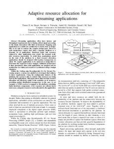
This is illustrated in Figure 1 where the guaranteed approximation factor γ is depicted versus the computational power, assuming that the base layer of the videos is at 100 kbps, there are K 0 = 1000 sub-requests in the queue, and that each iteration roughly takes 100 machine instructions to execute. According to Figure 1, a tracker with seed servers of total capacity 10 Mbps whose allocation is decided every second, can make sure that the approximation result is at least as good as 90% of the optimal if it can perform 10 giga low-level instructions per second.

Authorized licensed use limited to: SIMON FRASER UNIVERSITY. Downloaded on November 15, 2009 at 14:36 from IEEE Xplore. Restrictions apply.

Approximation factor γ

1

SRA GREEDY

0.8

0.6

0.4

0.2 0

5 Mbps seed 10 Mbps seed 15 Mbps seed 5 10 15 Computational power (GIPS)

20

Fig. 1. Tradeoff between approximation factor and computational complexity.

In sum, the SRA DP algorithm obtains answers very close to the optimal for small seeding capacities, but it has to sacrifice some non-negligible approximation factor for large seeding capacities. We propose another approximation algorithm for these cases in the next subsection. B. SRA GREEDY: Seed Resource Allocation using a Greedy Algorithm We present another approximation algorithm for the seed server allocation problem, whose running time is independent of the seeding capacity and only depends on the number of requests in the queue. We show that the result of this approximation gets very close to the optimal answer as the seeding capacity increases, e.g., C = 50 Mbps, though is worse than the algorithm SRA DP if the seeding capacity is small, e.g., C = 10 Mbps. Our approximation is based on relaxing the Integer Programming (IP) problem in Eq. (2) to its equivalent Linear Programming (LP) problem, in which the constraint (2c) is relaxed to (7a) and (7b). 0 ≤ x0k ≤ nk (1 ≤ k ≤ K) x0k ∈ R.

(7a) (7b)

In other words, we now allow a layer to be partially served, though it is not meaningful in practice. Having solved the LP problem in Eq. (7) and obtained the x0k values, we obtain a valid solution to the original IP problem by rounding down all x0k values: xk = bx0k c. Clearly, xk values form a valid answer for the IP form in Eq. (2), since they satisfy both constraints (2b) and (2c). We will see shortly that after this relaxation and down-rounding, how close the objective function (2a) will be to the optimal solution. The proposed algorithm is called SRA GREEDAY and is shown in Figure 2. Sub-requests are sorted in decreasing order of utility-to-cost ratio and are picked one by one in each iteration. Since some sub-requests are overlapping, i.e., each sub-request (k, j) is a subset of subrequests (k, j +1), . . . , (k, nk ), in each iteration we take those layers from sub-request (k, j) that are not already served by another sub-request (k, j 0 < j). The algorithm consists of sorting sub-requests, which runs in O(K 0 log K 0 ) where K 0 is

GreedyAllocation (K, C, n[], b[][], c[][]) 1. // K: number of requests, C: seeding capacity 2. // n[k]: number of sub-requests in the k-th requests (1 ≤ k ≤ K) 3. // b[k][j], c[k][j]: utility and cost of the j-th sub-request of the k-th request (1 ≤ j ≤ n[k]); b[k][0] and c[k][0] are assigned 0 4. // Output: x[]: number of sub-requests to serve from the k-th request PK // total number of sub-requests 5. K 0 = k=1 n[k] 6. S[] ←− the K 0 sub-requests sorted in decreasing order of utility-to-cost ratio 7. z ←− 0 // will be the total obtained utility 8. x[] ←− CreateArray(K, 0) 9. for (k, j) ∈ S do 10. if x[k] > j then continue 11. cost ←− c[k][j]−c[k][x[k]] 12. utility ←− b[k][j]−b[k][x[k]] 13. if cost ≤ C then 14. C ←− C − cost 15. z ←− z + utility 16. x[k] ←− j 17. done 18. return z, x[] Fig. 2.

A greedy algorithm for the seed server allocation problem.

the total number of sub-requests, and performing K 0 iterations of O(1), which makes the total running time O(K 0 log K 0 ). This is easily practical in real-time for reasonable K 0 values (< 500K). Theorem 3: If all costs ck,j are bounded as ck,j ≤ cmax < C for all valid k, j values, the algorithm SRA GREEDY is a cmax -factor approximation for the seed server allocation C − cmax cmax )OPT. problem, i.e., z ≥ (1 − C − cmax Proof: Consider the following two modifications to the algorithm in Figure 2: (i) after line 16 in the code, if cost > C then pick a portion θ (0 ≤ θ < 1) of the current sub-request (k, j) which can fill the capacity C, and quit the loop, (ii) after line 16 in the code, if cost > C then just quit the loop. Case (i) refers to the solution to the LP problem in Eq. (7) and provides the optimal answer for this problem; the proof is skipped as it is easy and similar to that of the solution to Knapsack’s LP-relaxation. Let z ∗ denote the utility obtained by this solution, which is at least as good as OPT since it refers to the LP-relaxation of the original problem. Case (ii) is only for a comparison purpose. Since its solution is a subset of the solution obtained by our algorithm in Figure 2, the utility obtained by case (ii), denoted by z 0 , is a lower bound on our obtained utility z, i.e., z 0 ≤ z.

Authorized licensed use limited to: SIMON FRASER UNIVERSITY. Downloaded on November 15, 2009 at 14:36 from IEEE Xplore. Restrictions apply.

Let m + 1 and m be the number of sub-requests taken by modifications (i) and (ii), respectively. Also let b1 , . . . , bm+1 and c1 , . . . , cm+1 be the short for the utilities and costs of these sub-requests. Since the m + 1-st sub-request served has a utility-to-cost ratio less than or equal to each of the previous m ones, we have: bi bm+1 ≤ for all i ∈ {1, 2, . . . , m} cm+1 ci Pm bm+1 i=1 bi ci ≤ bi ⇒ bm+1 ≤ cm+1 Pm (8) ⇒ cm+1 i=1 ci

¤

The margin between z and OPT is bounded as follows: z ≤ z 0 ≤ z ≤ OPT ≤ z ∗ ⇒ = 1 − OPT P P m bi + θbm+1 − m z0 z∗ − z0 i=1P i=1 bi 1− ∗ = = ≤ m z z∗ b + θb m+1 i=1 i Pm cmax b i=1 bi P 1 Pm+1 ≤ cm+1 Pm ≤ Pm ≤ m m b c b i=1 i i=1 i i=1 i i=1 ci cmax cmax ⇒ z ≥ (1 − ) OPT (9) C − cmax C − cmax

For example, for a 2 Mbps video and a seeding capacity of 25 Mbps, it is guaranteed that the greedy approximation solution will produce results as good as 91% of the optimal. For larger seeding capacities, this factor approaches 1. For small seeding capacities (≤ 10 Mbps), however, the approximation factor is low, e.g., 75% for C = 10 Mbps. In this case, employing the SRA DP algorithm is recommended as its factor is close to 1 for small seeding capacities. In sum, according to the seeding capacity, the computational power, and the maximum bitrate of the videos being served, one can determine the guaranteed approximation factor of both algorithms SRA DP and SRA GREEDY using Equations (6) and (9) choose the more appropriate one. C. The Utility Function The proposed allocation algorithms are general and can adopt different utility functions to suit the objective of various practical systems. In this section, we define a sample utility function, which is to provide max-min fairness among quality received by peers according to their demands. Let qp denote the quality, e.g., Y-PSNR, of the video that a peer p receives and dp denote the quality demand of peer p. Referring to the fraction qp /dp as peer satisfaction, the goal is to have those peers be served whose received quality is farthest from their demand (those with least satisfaction). That is, maximizing the minimum peer satisfaction. For example, if the resources in the network are half the total demanded, in the ideal case every peer should receive half of its demanded quality, not some peers completely satisfied and others starving. To achieve this, we define the utility function as: dp − q(vp , l − 1) (10) bself (p, l) = dp − q(vp , 0) where vp is the video being watched by peer p and q(vp , l) denotes the video quality added by the l-th layer of this

video. Notice that q(vp , 0) is also needed and thus needs to be realistically defined; note that a blank video can produce a Y-PSNR of 10 to 20 dB, depending on the original video. The q(vp , 0) value determines the importance of the base layer and does not considerably affect the way the enhancement layers are served in our algorithm: q(vp , 1) − q(vp , 0) can be defined superior to any other q(vp , l) − q(vp , l − 1) in order to make sure that everyone will receive the base layer. We set q(vp , 0) as 25 dB in our experiments in Section V. We now calculate the utilities bshare (p, l) according to the function bself (p, l) and peers upload bandwidths. As discussed earlier (Section III-B), bshare (p, l) refers to the expected utility gained by the system when peer p shares layer l with the network. Let Lp denote the number of layers that peer p demands. According to the way the peers are expected to share their upload bandwidth for serving different layers (Section III-B), we know the rate up,l at which a peer p will serve each layer l of video v: l−1 X © ª up,i , rv,l (1 ≤ l ≤ Lp ). up,l = min up −

(11)

i=1

If the upload bandwidth of peer p is higher than the bitrate of the demanded video, the bandwidth remained from Eq. (11) is equally divided among layers, P which adds to the right hand Lp rv,i )/Lp . side of Eq. (11) the term (up − i=1 Denote by Pv,l,p the set of peers who demand the video v at layers higher than or equal to l, and who can possibly be served by the peer p. Then, the function bshare (p, l) is calculated as: X ¡ ¢ up,l 1 × × bself (x, l)+bshare (x, l) . rv,l |Pv,l,p | x∈P v,l,p (12) Calculation of Eq. (12) for each peer is in the order of total number of peers for arbitrary bself (p, l) functions, which is not efficient. However, for specific cases such as providing max-min fairness, this can be estimated efficiently. Given the upload/download bandwidth distribution of peers, which can be obtained and updated during the streaming session, we can calculate the chance that a peer p’s layer demand Lp equals a given number l, to which we briefly refer as P r (l). This reduces the complexity of Eq. (12) from being in the order of number of peers to the order of number of video layers: bshare (p, l) =

L X up,l 1 i − q(vp , l − 1) . × PL P r (i) × rv,l i − q(vp , 0) P r (i) i=l i=l (13) In this calculations, a peer sharing data with its partners is taken into account, whereas further hops, i.e., those peers sharing, is not relied on, as it makes the accuracy of the calculated utilities very sensitive to network dynamics. Neglecting them, on the other hand, may underestimate the utility of peers sharing the layers, though underestimating the share utility similarly for all peers is more acceptable. At last, each of the bk,j values is calculated as:

bshare (p, l) =

Authorized licensed use limited to: SIMON FRASER UNIVERSITY. Downloaded on November 15, 2009 at 14:36 from IEEE Xplore. Restrictions apply.

1

70

0.95

Approximation ratio

Utility score

80

60 Optimal SRA DP SRA GREEDY FCFS BT-like

50

40 0

10

20 30 40 Time (minutes)

50

60

(a) Utility score.

0.85 0.8 0.75 0

10

20 30 40 Time (minutes)

50

60

(b) Gained utility over the maximum possible utility that can be gained. Fig. 3.

bk,j

SRA DP SRA GREEDY FCFS BT-like

0.9

Near-optimality of the proposed algorithms.

⎧ j=0 ⎪ ⎨ 0P reqk .l1 +j−1 ¡ = bself (reqk .p, l)+ l=reqk .l1 ⎪ ¢ ⎩ bshare (reqk .p, l) 1 ≤ j ≤ nk

(14)

V. E VALUATION

A. Simulation Setup We simulate on-demand distribution of a video file encoded in 10 quality layers at a bitrate of 2 Mbps, which a Y-PSNR quality of 27 dB to 40 dB. The video length is 7 minutes. We refer to the fraction of video quality received by a peer over its demanded quality as peer satisfaction. The objective of the system is to maximize the minimum peer satisfaction (max-min fairness), as discussed in Section IV-C. Peers join the network according to a Poisson distribution with expected 1 arrival per second. The network consists of 400–500 peers on average. The simulation runs for 60 minutes. Each peer, once finished watching the video, stays in the network for up to 3 minutes for serving others. Each peer may leave at any time according to an exponential probability distribution, by which 25% of peers leave the network before they finish watching the video and doing the expected seeding. For generating download and upload bandwidths of peers, two classes of peers are considered. The first class has 80% of peers and represents home users, which have download bandwidths between 100 kbps to 4 Mbps and upload bandwidth between 100 kbps to 1 Mbps. The second class has 20% of peers and represents campus users, which can have download and upload rates between 100 kbps to 4 Mbps. Each peer is thus capable of downloading and uploading the base layer at least. Each request of a peer to the tracker is first tried to be served by a list of potential senders. If there is no peer free to serve the requested layers, the requesting peer is served by the seed server. A peer might receive a layer from multiple peers, with the total receiving rate equal to the bitrate of the

layer. The seed server, on the other hand, only serves whole layers. The tracker gathers requests in its queue and runs the seed server allocation algorithm once every 10 seconds. In each such run, all streaming requests in the queue along with those that are currently being served are considered together and a new set of requests to be served is determined. Each sender peer disconnects its connection to a receiver according to a Bernoulli probability distribution with an expected value of 1 minute. This is done to make enough dynamics in the network and to simulate peer failures. Video segment length is assumed 10 seconds. The simulation runs following an eventdriven procedure with 10-second steps, i.e., events are gathered during a time step and applied at once the end. To avoid wide quality fluctuations at receiver side, we take a simple heuristic that does not allow more than 1 layer change in the number of layers in two consecutive segments, i.e., the heuristic at each peer drops the enhancement layers that violate this criterion. In addition to the proposed allocation algorithms, we consider two other algorithms: First-Come First-Serve (FCFS) and BitTorrent-like (BT-like). SRA DP, SRA GREEDY, and FCFS operate as follows. First, each requests in the ordered request queue is tried to be matched with available peers. The ordering of the request queue is based on the utility-to-cost ratio for SRA DP and SRA GREEDY, and based on arrival time of the requests in FCFS. After matching requests to available peers, a subset of the remaining requests is selected to be served according to the employed seed server allocation algorithm: SRA DP, SRA GREEDY, or serving in the order of arrival (FCFS). In the fourth method, BT-like, a different procedure is employed: requests are first responded by the seed servers in an FCFS manner, then the remaining requests are responded by a set of up to 30 randomly selected peers who do have the requested data but might not have enough available capacity. Being randomly selected to be served by a seed server might result in quality fluctuation at the receiving peer. Thus, a request that is randomly selected for serving is continuously served at least for 1 minute.

Authorized licensed use limited to: SIMON FRASER UNIVERSITY. Downloaded on November 15, 2009 at 14:36 from IEEE Xplore. Restrictions apply.

SRA GREEDY FCFS BT-like

Quality received (Y-PSNR)

Satisfaction factor

1

0.8

0.6

0.4

0.2 0

Fig. 4.

50 100 150 Seed servers capacity (Mbps)

200

Satisfaction experienced by at least 90% of peers.

B. Results We first evaluate how close the utility gained by different allocation methods is to the optimal. Figure 3 depicts the result of this evaluation. The optimal utility in this figure is calculated as follows. At each time step, we assume a virtual seed server that is formed by aggregating the capacity of all peers as well as the actual seed server, ignoring all data availability constraints at peers. Therefore, the optimal utility that can be gained using the virtual seed server is greater than or equal to the optimal utility that can be actually gained from the network. Since finding the optimal utility of the virtual seed server is an NP-complete problem (Theorem 1), we consider the optimal answer of the LP-relaxation of the problem, which is at least as large as the actual optimal utility; see Section IV-B. Thus, the optimal utility that we consider in Figure 3 is an upperbound on the maximum utility that can be gained in the network. Figure 3(a) shows how close the two proposed algorithms are to the optimal. This figure depicts the utility gained by the system (normalized to [0, 100]) over time using different seed server allocation algorithms. Figure 3(b) illustrates the near-optimality of our proposed algorithms. In this figure, the proposed algorithms SRA DP and SRA GREEDY always gain beyond 90% of the optimal with an average of 95%. The seed server capacity is 10 Mbps in Figures 3(a) and 3(b). The theoretical approximation ratio for this case is 96%, while we see it has reached slightly lower values in practice. This is due to dynamics of the network that were not involved in the approximation analyses, i.e., the experimental ratio would have been always higher that 96% if all peers stayed in the network as expected, they let the tracker (and the tracker was able to) decide and update their partnerships at every 10-second step, and all peers did obey our assumptions about sharing their upload bandwidths among layers, which we intentionally made them disobey by deviating by up to 50% from Eq. (11). Figure 3 also depicts that the two approximation algorithms operate almost equally efficiently for a seed server capacity of 10 Mbps; since the network consists of hundreds of peers we do not

34 2.1 dB

32

850 kbps

30 28 26 0

Fig. 5.

SRA GREEDY FCFS BT-like 1000 2000 3000 4000 Download bandwidth (kbps) Video quality for peers with different download bandwidths.

consider seeding capacities below 10 Mbps as such seed servers will not be realistic. For larger capacities, the dynamic algorithm takes a significant time to operate with reasonable approximation factor. Thus, we do not consider this method in next evaluations as they deal with large seeding capacities. We now evaluate the increase in the overall peer satisfaction, which is the fraction that a peer receives out of its demanded video quality. Figure 4 plots the satisfaction experienced by at least 90% of peers. The algorithm SRA GREEDY considerably increase the satisfactions especially for limited seeding capacities, which is often the case in practice. Figure 4 also shows that for a very large seeding capacity such as 200 Mbps, which is nearly enough for fully satisfying all peers even with the FCFS method, the BitTorrent-like method still could not increase the satisfaction as expected. That is because this method followed a random peer matching, which caused inefficient utilization of peers resources. Next, we evaluate the video quality delivered to peers. Figure 5 depicts the average Y-PSNR quality that peers with different download bandwidths could receive. The seed servers capacity is 25 Mbps in this figure. Without our algorithm, some higher quality levels could not be achieved at all (beyond 32 dB). The other quality levels would require peers to have a significantly larger bandwidth, e.g., beyond 2 Mbps for a quality of 32 dB whereas it is achieved by 1.2 Mbps by employing our algorithm. A quality increase of more than 2 dB is obtained for most peers; the quality range of the considered scalable video is 13 dB in total. Our algorithms rely on knowing and utilizing the upload bandwidth of peers. This could be a weakness if peers are not cooperative. However, Figure 6 reveals how peers are encouraged to cooperate: more cooperation will bring them a significantly higher quality. For example, peers who shared 2 Mbps upload bandwidth received a video quality of 36 dB on average, which is 2 dB higher that the quality received by those contributing 1 Mbps, and 5 dB higher than those contributing 250 kbps. One might argue that this result is because peers with higher upload bandwidth also have higher

Authorized licensed use limited to: SIMON FRASER UNIVERSITY. Downloaded on November 15, 2009 at 14:36 from IEEE Xplore. Restrictions apply.

provide a significantly higher video quality for those peers that upload more.

SRA GREEDY, 100 Mbps seed SRA GREEDY, 25 Mbps seed

R EFERENCES

FCFS, 100 Mbps seed FCFS, 25 Mbps seed

Quality received (Y-PSNR)

BT-like, 100 Mbps seed 38

BT-like, 25 Mbps seed

36 34 32 30 0

Fig. 6.

1000 2000 3000 Upload bandwidth (kbps)

4000

Incentive provided for peers to share upload bandwidth.

download bandwidth, and naturally receive more video layers. We see, however, that for methods FCFS and BT-like this quality difference is marginal; the received quality is almost independent of the upload bandwidth. Thus, the higher quality achieved by our allocation algorithms is due peers’ cooperation. With our algorithm compared to FCFS and BTlike algorithms, cooperating peers receive up to 7 dB higher quality, which is even more than half of the entire quality range of the video. This clearly shows the provided incentive for peers to cooperate as much as they can. VI. C ONCLUSION In this paper, we have considered streaming of scalable videos over P2P networks. In these networks, due to the asymmetry between peers download and upload bandwidths, a number of seed servers need to be deployed in the network for delivering high-quality videos to peers. We focused on the problem of allocating these seeding resources to peers in order to maximize a system-wide utility function. We formulated this problem and showed that it is NP-complete. We then proposed two approximation algorithms for the problem and proved that they produce near-optimal results. The first algorithm allocates seed servers based on dynamic programming and is preferred for limited seeding capacities (≤ 10 Mbps). The second algorithm is designed for larger capacities and follows a greedy approach. We evaluated the proposed algorithms by simulating a P2P streaming system. The results of our evaluations confirm that the utility obtained by the proposed algorithms is always beyond 90% of the optimal utility that can be gained from the system. The results show that the proposed seed server allocation algorithms result in peers receive more video layers, and thus an enhanced video quality (over 2 dB). Our algorithms also encourage peers to cooperate, as they

[1] “Global IPTV market analysis (2006-2010),” RNCOS, Tech. Rep., August 2006, http://www.rncos.com/Report/IM063.htm. [2] The Insight Research Corporation, “Streaming media, IPTV, and broadband transport: Telecommunications carriers and entertainment services 2006-2011,” 2006, http://www.insight-corp.com/execsummaries/ iptv06execsum.pdf. [3] “PPLive,” http://www.pplive.com/en/index.html. [4] “SopCast,” http://www.sopcast.org/. [5] “TVAnts,” http://www.tvants.com/. [6] X. Zhang, J. Liu, B. Li, and T. Yum, “CoolStreaming/DONet: a datadriven overlay network for peer-to-peer live media streaming,” in Proc. of IEEE INFOCOM’05, Miami, FL, March 2005, pp. 2102–2111. [7] X. Hei, C. Liang, J. Liang, Y. Liu, and K. Ross, “A measurement study of a large-scale P2P IPTV system,” IEEE Transactions on Multimedia, vol. 9, no. 8, pp. 1672–1687, December 2007. [8] B. Li and J. Liu, “Multirate video multicast over the Internet: An overview,” IEEE Network, vol. 17, no. 1, pp. 24–29, February 2003. [9] H. Schwarz, D. Marpe, and T. Wiegand, “Overview of the scalable video coding extension of the H.264/AVC standard,” IEEE Transactions on Circuits and Systems for Video Technology, vol. 17, no. 9, pp. 1103– 1120, September 2007. [10] M. Wien, H. Schwarz, and T. Oelbaum, “Performance analysis of SVC,” IEEE Transactions on Circuits and Systems for Video Technology, vol. 17, no. 9, pp. 1194–1203, September 2007. [11] T. Schierl, T. Stockhammer, and T. Wiegand, “Mobile video transmission using scalable video coding,” IEEE Transactions on Circuits and Systems for Video Technology, vol. 17, no. 9, pp. 1204–1217, September 2007. [12] O. Hillestad, A. Perkis, V. Genc, S. Murphy, and J. Murphy, “Adaptive H.264/MPEG-4 SVC video over IEEE 802.16 broadband wireless networks,” in Proc. of Packet Video Workshop (PV’07), Lausanne, Switzerland, November 2007, pp. 26–35. [13] Y. Liu, Y. Guo, and C. Liang, “A survey on peer-to-peer video streaming systems,” Peer-to-Peer Networking and Applications, vol. 1, no. 1, pp. 18–28, March 2008. [14] J. Liu, S. Rao, B. Li, and H. Zhang, “Opportunities and challenges of peer-to-peer Internet video broadcast,” Proceedings of the IEEE, vol. 96, no. 1, pp. 11–24, January 2008. [15] Y. Cui and K. Nahrstedt, “Layered peer-to-peer streaming,” in Proc. of ACM International Workshop on Network and Operating System Support for Digital Audio and Video (NOSSDAV’03), Monterey, CA, June 2003, pp. 162–171. [16] R. Rejaie and A. Ortega, “PALS: peer-to-peer adaptive layered streaming,” in Proc. of ACM International Workshop on Network and Operating System Support for Digital Audio and Video (NOSSDAV’03), Monterey, CA, June 2003, pp. 153–161. [17] M. Hefeeda and C. Hsu, “Rate-distortion optimized streaming of finegrained scalable video sequences,” ACM Transactions on Multimedia Computing, Communications and Applications, vol. 4, no. 1, pp. 2:1– 2:28, January 2008. [18] X. Lan, N. Zheng, J. Xue, X. Wu, and B. Gao, “A peer-to-peer architecture for efficient live scalable media streaming on Internet,” in Proc. of ACM Multimedia Conference, Augsburg, Germany, September 2007, pp. 783–786. [19] M. Zink, O. Kunzel, J. Schmitt, and R. Steinmetz, “Subjective impression of variations in layer encoded videos,” in Proc. of Workshop on Quality of Service (IWQoS’03), Berkeley, CA, June 2003, pp. 137–154. [20] X. Xiao, Y. Shi, and Y. Gao, “On optimal scheduling for layered video streaming in heterogeneous peer-to-peer networks,” in Proc. of ACM Multimedia Conference, Vancouver, BC, Canada, October 2008, pp. 785–788. [21] R. Rajendran and D. Rubenstein, “Optimizing the quality of scalable video streams on P2P networks,” Computer Networks, vol. 50, no. 15, pp. 2641–2658, October 2006. [22] D. Xu, M. Hefeeda, S. Hambrusch, and B. Bhargava, “On peer-topeer media streaming,” in Proc. of IEEE International Conference on Distributed Computing Systems (ICDCS’02), Vienna, Austria, July 2002, pp. 363–371. [23] H. Kellerer, U. Pferschy, and D. Pisinger, Knapsack Problems. Springer, 2004.

Authorized licensed use limited to: SIMON FRASER UNIVERSITY. Downloaded on November 15, 2009 at 14:36 from IEEE Xplore. Restrictions apply.