Efficient and Scalable MetaFeature-based Document Classification using Massively Parallel Computing
1
Sérgio Canuto1 , Marcos André Gonçalves1 , Wisllay Santos2 , Thierson Rosa2 , Wellington Martins2 Departament of Computer Science, Federal University of Minas Gerais, Belo Horizonte, Brazil {sergiodaniel,mgoncalv}@dcc.ufmg.br 3 Informatics Institute, Federal University of Goiás, Goiânia, Brazil {wisllaysantos,thierson,wellington}@inf.ufg.br
ABSTRACT The unprecedented growth of available data nowadays has stimulated the development of new methods for organizing and extracting useful knowledge from this immense amount of data. Automatic Document Classification (ADC) is one of such methods, that uses machine learning techniques to build models capable of automatically associating documents to well-defined semantic classes. ADC is the basis of many important applications such as language identification, sentiment analysis, recommender systems, spam filtering, among others. Recently, the use of meta-features has been shown to substantially improve the effectiveness of ADC algorithms. In particular, the use of meta-features that make a combined use of local information (through kNN-based features) and global information (through category centroids) has produced promising results. However, the generation of these meta-features is very costly in terms of both, memory consumption and runtime since there is the need to constantly call the kNN algorithm. We take advantage of the current manycore GPU architecture and present a massively parallel version of the kNN algorithm for highly dimensional and sparse datasets (which is the case for ADC). Our experimental results show that we can obtain speedup gains of up to 15x while reducing memory consumption in more than 5000x when compared to a state-of-the-art parallel baseline. This opens up the possibility of applying meta-features based classification in large collections of documents, that would otherwise take too much time or require the use of an expensive computational platform.
Keywords document classification, meta-features, parallelism
1.
INTRODUCTION
The processing of large amounts of data efficiently is critical for Information Retrieval (IR) and, as this amount of Permission to make digital or hard copies of all or part of this work for personal or classroom use is granted without fee provided that copies are not made or distributed for profit or commercial advantage and that copies bear this notice and the full citation on the first page. Copyrights for components of this work owned by others than ACM must be honored. Abstracting with credit is permitted. To copy otherwise, or republish, to post on servers or to redistribute to lists, requires prior specific permission and/or a fee. Request permissions from
[email protected]. SIGIR ’15 August 09 - 13, 2015, Santiago, Chile Copyright 2015 ACM 978-1-4503-2782-4/14/04 ...$15.00. http://dx.doi.org/10.1145/2766462.2767743.
data grows, storing, indexing and searching costs rise up altogether with penalties in response time. Parallel computing may represent an efficient solution for enhancing modern IR systems but the requirements of designing new parallel algorithms for modern platforms such as manycore Graphical Processing Units (GPUs) have hampered the exploitation of this opportunity by the IR community. In particular, similarity search is at the heart of many IR systems. It scores queries against documents, presenting the highest scoring documents to the user in ranked order. The kNN algorithm is commonly used for this function, retrieving the most similar k documents for each query. Another very common application domain for kNN is Automatic Document Classification (ADC). In this case, the kNN algorithm is used to automatically map (classify) a new document d to a set of predefined classes given a set of labeled (training) documents, based on the similarities between d and each of the training docoments. kNN has been shown to produce competitive results in several datasets [15]. The speedup of this type of algorithm, using some efficient parallel strategies, mainly in applications in which it is repetitively applied as the core of other applications, opens huge opportunities. One recent application which uses kNN intensively is the generation of meta-level features (or simply meta-features) for ADC [21]. Such meta-features capture local and global information about the likelihood of a document to belong to a class, which can then be exploited by a different classifier (e.g. SVM). More specifically, meta-features capture: (i) the similarity value between a test example and the nearest neighbor in each considered class, and (2) the similarity value of the test example with the classes’ centroids 1 . As shown in [21] and in our experiments, the use of metafeatures can substantially improve the effectiveness of ADC algorithms. However, the generation of meta-features is very costly in terms of both, memory consumption and runtime. In order to generate them, there is the need to constantly call the kNN algorithm. kNN, however, is known to produce poor performance (execution time) in classification tasks in comparison to other (non-lazy) supervised methods, normally being not the best choice to deal with on-the-fly classifications. Classification using kNN-based meta-features inherits this poor performance, since we need to generate meta-level features for both, all training, and each new test sample before actual classification. For textual datasets (with large 1 Notice that this also has to be applied to all training documents in an offline procedure.
vocabularies), the performance problem is hardened, since the kNN algorithm will have to run on high dimensional data. In this scenario, kNN often requires large portions of memory to represent all the training data and intensive computation to calculate the similarity between points. In fact, as we shall see the generation of meta-features is not feasible using previous meta-feature generators [5, 21] for the larger datasets we experimented with. In this paper we present a new GPU-based implementation of kNN specially designed for high-dimensional and sparse datasets (which is the case for ADC), allowing a very fast and much more scalable meta-feature generation which allows one to apply this technique in large collections much faster. Some of the most interesting characteristics of our approach, compared to other state-of-the-art GPU-based proposals, include: • most solutions use a brute-force approach (i.e., compare the query document to all training documents) which demands too much memory while we exploit inverted indexes along with an efficient implementation to cope with GPU memory limitations; • in order to scale, some solutions sacrifice effectiveness using an approximated kNN solution (e.g. localitysensitive hashing - LSH) while our proposal is an exact kNN solution which exploits state-of-the-art GPU sorting methods; • most proposals achieve good results only when considering many queries (i.e., multiple document classification) in order to produce good speedups while our solution obtains improvements even when dealing with a single query (document); we achieve this by an effective load balacing approach within the GPU; • some solutions require a multi-GPU approach to deal with large datasets while ours deals with large datasets using a single GPU. Our experimental results show that we can obtain speedup gains of up to 140x and 15x while reducing memory consumption in more than 8000x and 5000x when compared to a standard sequential implementation and to a state-of-theart parallel baseline, respectively. This paper is organized as follows. Section 2 covers related work. Section 3 introduces the use of meta-feature in ADC. Section 4 provides a brief introduction to parallelism in GPU. Section 5 describes our GPU-based implementation, specially designed for highly dimensional, sparse data. Section 6 presents an analysis of the complexity of the proposed solution. Section 7 presents our experimental evaluation while Section 8 concludes the paper.
2.
RELATED WORK
Several meta-features have been proposed to improve the effectiveness of machine learning methods. They can be based on ensemble of classifiers [2, 20], derived from clustering methods [9, 14] or from the instance-based kNN method [5, 21]. Meta-features derived from ensembles exploit the probability distribution over all classes generated by each of the individual classifiers composing the ensemble [20]. In [2] other ensemble-based meta-features were also used, including: the entropies of the class probability distributions and
the maximum probability returned by each classifier. This scheme was found to perform better than using only probability distributions. Clustering techniques may also be used to derive metafeatures. In this case, the feature space is augmented using clusters derived from a previous clustering step considering both the labeled and unlabeled data [14, 9]. The idea is that clusters represent higher level “concepts” in the feature space, and the features derived from the clusters indicate the similarity of each example to these concepts. In [14] the largest n clusters are chosen as representatives of the major concepts. Each cluster c contributes with a set o meta-features like, for instance, binary feature indicating if c is the closest of the n clusters to the example, the similarity of the example to the cluster’s centroid, among others. In [9] the number of clusters is chosen to be equal to the predefined number of classes and each cluster corresponds to an additional meta-feature. Recently, [5] reported good results by designing metafeatures that make a combined use of local information (through kNN-based features) and global information (through category centroids) in the training set. Despite the fact that these meta-features are not created based on an ensemble of classifiers, they differ from the previously presented metafeatures derived from clusters because they explicitly capture information from the labeled set. Although the kNN algorithm can be applied broadly, it has some shortcomings. For large datasets (n) and high dimensional space (d), its complexity O(nd) can easily become prohibitive. Moreover, if m successive queries are to be performed, the complexity further increases to O(mnd). Recently, some proposals have been presented to accelerate the kNN algorithm via a highly mutithreaded GPU-based approach. The first, and most cited, GPU-based kNN implementation was proposed by Garcia et al. [3]. They used the brute force approach and reported speedups of up to two orders of magnitude when compared to a brute force CPUbased implementation. Their implementation assumes that multiple queries are performed and computes and stores a complete distance matrix, what makes it impracticable for large data (over 65,536 documents). Following Garcia’s et al. work, Kuang and Zhao [8] implemented their own optimized matrix operations for calculating the distances, and used radix sort to find the top-k elements. Liang et al. [12] took advantage of CUDA Streams to overlap computation and communication (CPU/GPU) when dealing with several queries, and thus decrease the GPU memory requirements. The distances were computed in blocks and later merged first locally and then globally to find the top-k elements. However, such works can still be considered brute-force. Sismanis et al. [18] concentrated on the sorting phase of the brute-force kNN and provided an extensive comparison among parallel truncated sorts. They conclude that the truncated biotonic sort (TBiS) produces the best results. Our proposal differs from the above mentioned work in many aspects. First, it exploits a very efficient GPU implementation of inverted indexes which supports an exact kNN solution without relying in brute-force. This also allows our solution to save a lot of memory space since the inverted index corresponds to a sparse representation of the data. In the distance calculation step, we resort to a smart load balancing among threads to increase the parallelism. And in
the sorting step, we exploit a GPU-based sorting procedure, which was shown to be superior to other partial sorting algorithms[18], in combination with a CPU merge operation based on a priority queue.
3.
USE OF META-FEATURES FOR ADC
In here, we formally introduce the meta-features whose kNN-based calculation we intend to speed up and scale with our proposed massively parallel approach. Let X and C denote the input (feature) and output (class) spaces, respectively. Let Dtrain = {(xi , ci ) ∈ X × C}|n i=1 be the training set. Recall that the main goal of supervised classification is to learn a mapping function h : X 7→ C which is general enough to accurately classify examples x0 6∈ Dtrain . The kNN-based meta-level features proposed in [5], are designed to replace the original input space X with a new informative and compact input space M. Therefore, each vector of meta-features mf ∈ M is expressed as the concatenation of the sub-vectors below, which are defined for each example xf ∈ X and category cj ∈ C for j = 1, 2, . . . , |C| as: • ~v~xcos = [cos(~xij , x~f )]: A k-dimensional vector produced f by considering the k nearest neighbors of class cj to the target vector xf , i.e., , ~ xij is the ith (i ≤ k) nearest neighbor to ~xf , and cos(~ xij , x~f ) is the cosine similarity between them. Thus, k meta-features are generated to represent xf . • ~v~xLf1 = [d1 (~xij , x~f )]: A k-dimensional vector whose elements d1 (~xij , ~ xf ) denote the L1 distance between ~ xf and the ith nearest class cj neighbor of ~ xf (i.e., d1 (~xij , ~xf ) = ||~ xij − ~ xf ||1 ). • ~vxL~f2 = [d2 (~xij , x~f )]: A k-dimensional vector whose elements d2 (~xij , x~f ) denote the L2 distance between ~ xf and the ith nearest class cj neighbor of x~f (i.e., d2 (~xij , x~f ) = ||~ xij − x~f ||2 ). = [d2 (~xj , x~f ), cos(~ xj , x~f )]: A 2-dimensional vec• ~vxcent ~f tor where ~xj is the cj centroid (i.e., vector average of all training examples of the class cj ). Considering k neighbors, the number of features in vector xf is (3k + 2) per category, and the total of (3k + 2)|C| for all categories. The size of this meta-level feature set is much smaller than that typically found in ADC tasks, while explicitly capturing class discriminative information from the labeled set.
4.
PARALLELISM AND THE GPU
In the last few years, the focus on processor architectures has moved from increasing clock rate to increasing parallelism. Rather than increasing the speed of its individual processor cores, traditional CPUs are now virtually all multicore processors. In a similar fashion, manycore architectures like GPUs have concentrated on using simpler and slower cores, but in much larger counts, in the order of thousands of cores. The general perception is that processors are not getting faster, but instead are getting wider, with an ever increasing number of cores. This has forced a renewed interest in parallelism as the only way to increase performance. The high computational power and affordability of GPUs has led to a growing number of researchers making use of
GPUs to handle massive amounts of data. While multicore CPUs are optimized for single-threaded performance, GPUs are optimized for throughput and a massive multi-threaded parallelism. As a result, the GPUs deliver much better energy efficiency and achieves higher peak performance for throughput workloads. However, GPUs have a different architecture and memory organization and to fully exploit its capabilities it is necessary considerable parallelism (tens of thousands of threads) and an adequate use of its hardware resources. This imposes some constraints in terms of designing appropriate algorithms, requiring the design of novel solutions and new implementation approaches. However, a few research groups and companies have faced this challenge with promising results in Database Scalability, Document Clustering, Learning to Rank, Big Data Analytics and Interactive Visualization [1, 19, 17, 13, 6]. The GPU consists of a M-SIMD machine, that is, a Multiple SIMD (Single Instruction Multiple Data) processor. Each SIMD unit is known as a streaming multiprocessor (SM) and contains streaming processor (SP) cores. At any given clock cycle, each SP executes the same instruction, but operates on different data. The GPU supports thousands of light-weight concurrent threads and, unlike the CPU threads, the overhead of creation and switching is negligible. The threads on each SM are organized into thread groups that share computation resources such as registers. A thread group is divided into multiple schedule units, called warps, that are dynamically scheduled on the SM. Because of the SIMD nature of the SP’s execution units, if threads in a schedule unit must perform different operations, such as going through branches, these operations will be executed serially as opposed to in parallel. Additionally, if a thread stalls on a memory operation, the entire warp will be stalled until the memory access is done. In this case the SM selects another ready warp and switches to that one. The GPU global memory is typically measured in gigabytes of capacity. It is an off-chip memory and has both a high bandwidth and a high access latency. To hide the high latency of this memory, it is important to have more threads than the number of SPs and to have threads in a warp accessing consecutive memory addresses that can be easily coalesced. The GPU also provides a fast on-chip shared memory which is accessible by all SPs of a SM. The size of this memory is small but it has a low latency and it can be used as a softwarecontrolled cache. Moving data from the CPU to the GPU and vice versa is done through a PCIExpress connection. The GPU programming model requires that part of the application runs on the CPU while the computationallyintensive part is accelerated by the GPU. The programmer has to modify his application to take the compute-intensive kernels and map them to the GPU. A GPU program exposes parallelism through a data-parallel SPMD (Single Program Multiple Data) kernel function. During implementation, the programmer can configure the number of threads to be used. Threads execute data parallel computations of the kernel and are organized in groups called thread blocks, which in turn are organized into a grid structure. When a kernel is launched, the blocks within a grid are distributed on idle SMs. Threads of a block are divided into warps, the schedule unit used by the SMs, leaving for the GPU to decide in which order and when to execute each warp. Threads that belong to different blocks cannot communicate explicitly and have to rely on the global memory to share their
results. Threads within a thread block are executed by the SPs of a single SM and can communicate through the SM shared memory. Furthermore, each thread inside a block has its own registers and private local memory and uses a global thread block index, and a local thread index within a thread block, to uniquely identify its data.
Algorithm 1: CreateInvetedIndex(E) input : term-document pairs in E[ 0 . . |E| − 1 ]. output: df , index, norms, invertedIndex. 1 2 3 4
5.
GPU-BASED GENERATION OF METAFEATURES
The proposed parallel implementation, called GPU-based Textual kNN (GT-kNN), greatly improves the k nearest neighbors search in textual datasets. The solution efficiently implements an inverted index in the GPU, by using a parallel counting operation followed by a parallel prefix-sum calculation, taking advantage of Zipf’s law, which states that in a textual corpus, few terms are common, while many of them are rare. This makes the inverted index a good choice for saving space and avoiding unnecessary calculations. At query time, this inverted index is used to quickly find the documents sharing terms with the query document. This is made by constructing a query index which is used for a load balancing strategy to evenly distribute the distance calculations among the GPU’s threads. Finally, the k nearest neighbors are determined through the use of a truncated bitonic sort to avoid sorting all computed distances. Next we present a detailed description of these steps.
5.1
5 6 7 8 9 10 11
12 13 14
Creating the Inverted Index
The inverted index is created in the GPU memory, assuming the training dataset fits in memory and is static. Let V be the vocabulary of the training dataset, that is the set of distinct terms of the training set. The input data is the set E of distinct term-documents (t, d), pairs occurring in the original training dataset, with t ∈ V and d ∈ Dtrain . Each pair (t, d) ∈ E is initially associated with a term frequency tf , which is the number of times the term t occurs in the document d. An array of size |E| is used to store the inverted index. Once the set E has been moved to the GPU memory, each pair in it is examined in parallel, so that each time a term is visited the number of documents where it appears (document frequency - df ) is incremented and stored in the array df of size |V|. A parallel prefix-sum is executed, using the CUDPP library [16], on the df array by mapping each element to the sum of all terms before it and storing the results in the index array. Thus, each element of the index array points to the position of the corresponding first element in the invertedIndex, where all (t, d) pairs will be stored ordered by term. Finally, the pairs (t, d) are processed in parallel and the frequency-inverse document frequency tf -idf (t, d) for each pair is computed and included together with the documents identification in the invertedIndex array, using the pointers provided by the index array. Also during this parallel processing, the value of the norm for each training document, which is used in the calculus of the cosine or Euclidean distance, is computed and stored in the norms array. Algorithm 1 depicts the inverted index creation process. Figure 1 illustrates each step of the inverted index creation for a five documents collection where only five terms are used. If we take t2 as an example, the index array indicates that its inverted document list (d2 , d4 ) starts at position 3 of the invertedindex array and finishes at position 4 (5 minus 1).
array of integers df [ 0 . . |V| − 1 ] // document-frequency array, initialized with zeros. array of integers index[ 0 . . |V| − 1 ]. array of floats norms[ 0 . . |Dtrain − 1| ]. invertedIndex[ 0 . . |E| − 1 ] // the inverted index Count the occurrences of each term in parallel on the input and accumulates in df . Perform an exclusive parallel prefix sum on df and stores the result in index. Access in parallel the pairs in E, with each processor performing the following tasks: begin Compute the tf-idf value of each pair. Accumulate the square of the tf-idf value of a pair (t, d) in norms[d]. Store in invertedIndex the entries corresponding to pairs in E, according to index. end Compute in parallel the square root of the values in array norms. Return the arrays: count, index, norms and invertedIndex.
d1
t1
t3
d2
t2
t5
d3
t1
d4
t2
d5
t1
t4
E (entries) 7 8 2 3 4 5 6 9 0 1 d1 d1 d1 d2 d2 d3 d4 d5 d5 d5 t1 t3 t4 t2 t5 t1 t2 t1 t3 t5 2 0 3 4 1 t1 t2 t3 t4 t5 3 1 2 2 2 df
t3
t5
Document Collection
2 0 3 4 1 t1 t2 t3 t4 t5 0 7 8 3 5 index
Count number of terms
Compute prefix sum
Point to 1st positions
7 8 2 3 5 6 9 0 4 1 t1 t1 t1 t2 t2 t3 t3 t4 t5 t5 d1 d3 d5 d2 d4 d1 d5 d1 d2 d5 invertedIndex
Figure 1: Creating the inverted index
5.2
Calculating the distances
Once the inverted index has been created, it is now possible to calculate the distances between a given query document q and the documents in Dtrain . The distances computation can take advantage of the inverted index model, because only the distances between query q and those documents in Dtrain that have terms in common with q have to be computed. These documents correspond to the elements of the invertedIndex pointed to by the entries of the index array corresponding to the terms occurring in the query q. The obvious solution to compute the distances is to distribute the terms of query q evenly among the processors and let each processor p access the inverted lists corresponding to terms allocated to it. However, the distribution of terms in documents of text collections is known to follow approximately the Zipf Law. This means that few terms occur in large amount of documents and most of terms occur in only few documents. Consequently, the sizes of the inverted list also vary according to te Zipf Law, thus distributing the work load according to the terms of q could cause a great imbalance of the work among the processors.
In this paper besides using an inverted index to boost the computation of the distances, we also propose a load balance method to distribute the documents evenly among the processors so that each processor computes approximately the same number of distances. In order to facilitate the explanation of this method, suppose that we concatenate all the inverted lists corresponding to terms in q in a logical vector Eq = [ 0 . . |Eq | − 1 ], where |Eq | is the sum of the sizes of all inverted lists of terms in q. Considering the example in Fig. 1 and supposing that q is composed by the terms t1 , t3 and t4 , the logical vector Eq would be formed by the following pairs of the inverted index: Eq = [(t1 , d1 ), (t1 , d3 ), (t1 , d5 ), (t3 , d1 ), (t3 , d5 ), (t4 , d1 )] and |Eq | equals to six. Given a set of processors P = {p0 , · · · p|P|−1 }, the load balance method should allocate elements of Eq in intervals of approximately the same size, that is, each processor pi ∈ P should process elements of Eq in the interval |E | |E | [id |P|q e, min((i + 1)d |P|q e − 1, |Eq | − 1)]. Consider de example stated above, and suppose that the set of processors is P = {p0 , p1 , p2 }. Thus elements of Eq with indices in the interval [0, 1] would be assigned to p0 , indices in [2, 3] would be processed by p1 and indices in [4, 5] would be processed by p2 . Since each processor knows the interval of the indices of the logical vector Eq it has to process, all that is necessary to execute the load balancing is a mapping of the logical indices of Eq to the appropriate indices in the inverted index (array invertedIndex). In the case of the example associated to Fig. 1, the following mappings between logical indices and indices of the invertedIndex array must be performed: 0 → 0, 1 → 1, 2 → 2, 3 → 5, 4 → 6 and 5 → 7. Each processor executes the mapping for the indices in the interval corresponding to it and finds the corresponding elements in the invertedIndex array for which it has to compute the distances to the query. Let Vq ⊂ V be the vocabulary of the query document d. The mapping proposed in this paper uses three auxiliary arrays: dfq [ 0 . . |Vq | − 1 ], startq [ 0 . . |Vq | − 1 ]] and indexq [ 0 . . |Vq | − 1 ]. The arrays dfq and startq are obtained together by copying in parallel df [ti ] to dfq [ti ] and index[ti ] to startq [ti ], respectively, for each term ti in the query q. Once the dfq is obtained, an inclusive parallel prefix sum on dfq is performed and the results are stored in indexq . Algorithm 2 shows the pseudo-code for the parallel computation of the distances between documents in the training set and the query document. In lines 4-7 the arrays dfq and startq are obtained. In line 8 the array indexq is obtained by applying a parallel prefix sum on array dfq . Next, each processor executes a mapping of each position x in the interval of indices of Eq associated to it to the appropriate position of the invertedIndex. This mapping is described in lines 10-17 of the algorithm. Then, the mapped entries of the inverted index are used to compute the distances between each document associated with these entries and the query. Figure 2 illustrates each step of Algorithm 2 for a query containing three terms, t1 , t3 and t4 , using the same collection presented in the example of Figure 1. Initially, the arrays dfq and startq are obtained by copying in parallel entries respectively from arrays df and index, corresponding to the three query terms. Next a parallel prefix sum is applied to array dfq and the indexq array is obtained. Finally the Figure shows the mapping of each position of the logical ar-
Algorithm 2: DistanceCalculation(invertedIndex, q) input : invertedIndex, df , index, query q[ 0 . . |Vq | − 1 ]. output: distance array dist[ 0 . . |Dtrain | − 1 ] initialized according to the distance function used. 1 2 3 4 5 6 7 8 9 10
11 12 13 14 15 16 17 18
19 20
array of integers dfq [ 0 . . |Vq | − 1 ] initialized with zeros array of integers indexq [ 0 . . |Vq | − 1 ] array of integers startq [ 0 . . |Vq | − 1 ] for each term ti ∈ q, in parallel do dfq [i] = df [ti ]; startq [i] = index[ti ]; end Perform an inclusive parallel prefix sum on dfq and stores the results in indexq foreach processor pi ∈ P do |Eq | |Eq | for x ∈ [id |P| e, min((i + 1)d |P| e − 1, |Eq | − 1)] do // Map position x to the correct position indInvP os of the invertedIndex pos = min(i : indexq [i] > x); if pos = 0 then p = 0; of f set = x; else p = indexq [pos − 1]; of f set = x − p; end indInvP os = startq [pos] + of f set uses q[pos] and invertedIndex[indInvP os] in the partial computation of the distance between q and the document associated to invertedIndex[indInvP os] end end
q 2 0 3 4 1 t1 t2 t3 t4 t5 0 7 8 3 5 index 0
t1
0
t3
2
1 5
t4
7 startq
t1
t3
t4 query
Parallel copy
2 0 3 4 1 t1 t2 t3 t4 t5 3 1 2 2 2 df
2 0 1 t1 t3 t4 3 2 1 dfq
2 0 1 t1 t3 t4 3 5 6 indexq
2 3 5 0 4 1 t1 t1 t1 t3 t3 t4 Logical array d1 d3 d5 d1 d5 d1 Eq 7 8 2 3 5 6 9 0 4 1 t1 t1 t1 t2 t2 t3 t3 t4 t5 t5 d1 d3 d5 d2 d4 d1 d5 d1 d2 d5 invertedIndex
Figure 2: Example of the execution of Algorithm 2 for a query with three terms.
ray Eq into the corresponding positions of the invertedIndex array.
5.3
Finding the k Nearest Neighbors With the distances computed, it is necessary to obtain the k closest documents. This can be accomplished by making use of a partial sorting algorithm on the array containing the distances, which is of size |Dtrain |. For this, we implemented a parallel version of the Truncated Bitonic Sort (TBiS), which was shown to be superior to other partial sorting algorithms in this context [18]. One advantage of the parallel TBiS is data independence. At each step, the algorithm distributes elements equally among the GPU’s threads
avoiding synchronizations as well as memory access conflicts. Although the partial bitonic sort is O(|Dtrain | log2 k), worse than the best known algorithm which is O(|Dtrain | log k), for a small k the ratio of log k becomes almost negligible. In the case of ADC using kNN, the value of k is usually not greater than 50. Our parallel TBiS implementation also uses a reduction strategy, allowing each GPU block to act independently from each other on a partition of array containing the computed distances. Results are then merged in the CPU using a priority queue.
6.
ANALYSIS OF THE SOLUTION
In this section we analyze the amount of time and memory used to construct the index and to compute the k nearest neighbors for a given query document q. The first step of the construction of the inverted index is to obtain the df array (line 5 of the Algorithm 1). During this step, the set of input pairs E is read in parallel by all processors in P and for each term the corresponding document |E| ). The parcounter is incremented. This takes time O( |P| allel prefix sum algorithm applied to array df to obtain the |V| index takes time O( |P| log |V|) [16]. Next, the computation of tf -idf , the computation of accumulated square of tf -idf (to compose the norms of the documents), and the insertion of pairs in the invertedIndex (lines 9-11) are done by accessing elements of E in parallel, thus taking time |E| ). Finally the square roots of the norms are computed O( |P| train | in time O( |D|P| ). The total time of the index construction
|E| |V| |E| train | is O( |P| ) + O( |P| log |V|) + O( |P| ) + O( |D|P| ). Since in real text collections |E| > |Dtrain | > |V|, we conclude that the |E| time complexity of the index construction is O( |P| ). The computation of the distances between each training document and the query document q starts by obtaining the arrays dfq and startq (lines 4-7 of Algorithm 2). This step is executed in parallel by all processors in P. Thus the two |Vq | arrays are computed in time O( |P| ). The computation of array indexq is the result of the use of the parallel prefix |Vq | sum on array dfq , thus it is done in time O( |P| log |Vq |). |E |
Each processor pi ∈ P executes the mapping of |P|q positions of the logical array Eq . It is possible to estimate the value of |Eq | in terms of the sizes of V and Vq . Remember that the logical array Eq represents the concatenation of all inverted lists of terms in the query document q, that is, |Vq | inverted lists. Considering that the training collection follows the Zipf Law, we have that the probability of the occurrence of a term t with rank k is given k−s by P|V| , where s is the value of the exponent charac1 i=1 is
terizing the distribution. The term with greatest probability is the term with rank 1. Thus the expected document |E| frequency of this term is given by P|V| . If we use the 1 i=1 is
classic version of Zipf’s law, the exponent s is 1, then the |E| document frequency of this term is P|V| ≈ ln|E| . This 1 |V| i=1 i
value represents an upper bound for lengths of the document frequency of each term in q. Thus, in the worst case, we have that |Eq | ≈ |Vq | ln|E| . According to Heaps Law, the |V| size of vocabulary is |V| = k|W |β , where k is a constant, usually in the range 10-100, W is the set formed by all occurrences of all terms in the collection, and β is another
constant in the range 0.4-0.6. The size of W can be taken as an upper bound for the size of the input pairs E. Thus |W | | ) = O(|Vq |). |Eq | = O(|Vq | log (k|W ) = O(|Vq | |W |β|Wlog |β ) β k β We conclude that and each processor pi executes the map|Vq | ping of O( |P| ) positions. Now we analyze the time to compute the mapping of a single position (lines 11-17 of Algorithm 2). The computing of variable pos in line 11 can be performed in time O(log |Vq |) because values in array dfq are disposed in ascending order and a binary search can be used to find the minimum index required. All the remaining operations (lines 12-18) are computed in constant time (O(1)). The processing of each mapped pair of the inverted index, as part of the computation of the distance between q and the corresponding document in the pair, is also done in constant time. Thus, the execution time of one iteration of inner loop (lines 10-18) is O(log |Vq |) + O(1) = O(log |Vq |). Finally the partial sort of the distances is computed in time O(|Dtrain | log k). Consequently, the overall execution time of Algorithm 2 corre|Vq | |Vq | |Vq | ) + O( |P| log |Vq |) + O( |P| )(O(log |Vq |)+ sponds to O( |P| |V |
q )(O(log |Vq |) + O(|Dtrain | log k). O(|Dtrain | log k) = O( |P| The work of Garcia et al.[3] processes many query documents in parallel, however, each query q is compared to every document in the training set. Besides, the query and each document are represented as arrays of sizes |V|. Thus, the processing time of query q is O(|V||Dtrain |)+O(|Dtrain | log k). When Comparing the speedup of our solution over the Garcia’s algorithm we do not take into consideration the time to sort the array of distances, since this task ads the same computing time in both solution. As consequence the O(|V||Dtrain |) . If we take |V| as upspeedup achieved is |Vq |
O( |P| )(O(log |Vq |)
per bound for |Vq |, we have that the speedup obtained is: speedup = O(
|Dtrain ||P| ) log |V|
If we consider that number of processors is constant (in one GPU), and that, according to Heaps Law the number of new words in vocabulary V does not grow much as the collection size increases, we have that, the speedup increases proportionally to the number of documents in the collection. Considering memory space requirements, the proposed solution consumes 2|E| units of memory to store arrays E and invertedIndex, consumes 2|V| units to store arrays df and index, consumes O(|Vq |) space to store the related-to-query arrays (dfq , startq , and indexq ) and O(|Dtrain |) space to store the array containing the norms of the documents and the array containing the distances. Thus, the space complexity of the solution is O(|E|)+O(|V|)+O(|Vq |)+O(|Dtrain |) = O(|E|) + O(|Dtrain |). The solution presented by Garcia et al. [3] uses a matrix with dimensions |V||Dtrain | to store the training set and an array of size |V| to store the query q. Thus the space complexity of their solution is O(|V||Dtrain |) + O(|Dtrain |). The ratio between the space used by Garcia’s solution and ours train | ). This corresponds to a mesure of the solution is O( |V||D (|E|) sparsity of the matrix storing the training set in Garcia’s solution.
7.
EXPERIMENTAL EVALUATION
7.1
Experimental Setup
In order to evaluate the meta-feature strategies, we consider six real-world textual datasets, namely, 20 Newsgroups, Four Universities, Reuters, ACM Digital Library, MEDLINE and RCV1 datasets. For all datasets, we performed a traditional preprocessing task: we removed stopwords, using the standard SMART list, and applied a simple feature selection by removing terms with low “document frequency (DF)”2 . Regarding term weighting, we used TFIDF for both, SVM and kNN. All datasets are single-label. In particular, in the case of RCV1, the original dataset is multi-label with the multi-label cases needing special treatment, such as score thresholding, etc. (see [11] for details). As our current focus is on single-label tasks, to allow a fair comparison among the other datasets (which are also single-label) and all baselines (which also focus on single-label tasks), we decided to transform all multi-label cases into single-label ones. In order to do this fairly, we randomly selected, among all documents with more than one label, a single label to be attached to that document. This procedure was applied in about 20% of the documents of RCV1 which happened to be multi-label. More details about the datasets are shown in Table 1. Dataset
Classes
# attrib
# docs
Density
Size
4UNI
7
40,194
8,274
140.325
14MB
20NG
20
61,049
18,766
130.780
30MB
ACM
11
59,990
24,897
38.805
8.5MB
REUT90
90
19,589
13,327
78.164
13MB
MED
7
803,358
861,454
31.805
327MB
RCV1Uni
103
134,932
804,427
79.133
884MB
Table 1:
General information on the datasets.
R All experiments were run on a Intel i7-870, running at 2.93GHz, with 16Gb RAM. The GPU experiments were run on a NVIDIA Tesla K40, with 12Gb RAM. In order to consider the costs of all data transfers in our efficiency experiments, we report the wall times on a dedicated machine so as to rule out external factors, like high load caused by other processes. To compare the average results on our crossvalidation experiments, we assess the statistical significance of our results with a paired t-test with 95% confidence and Bonferroni correction to account for multiple tests. This test assures that the best results, marked in bold, are statistically superior to others. We compare the computation time to generate meta-features using three different algorithms: (1) GTkNN, our GPUbased implementation of kNN3 ; (2) BF-CUDA, a brute force kNN implementation using CUDA proposed by Garcia et al. [3]; and (3) ANN, a C++ library that supports exact and approximate nearest neighbor searching4 . We use the ANN exact version, since it was used in the previous meta-feature works [5, 21]. We chose BF-CUDA because it is the main representative of the GPU-based brute force ap-
2
We removed all terms that occur in less than six documents (i.e., DF