Scalable Techniques for Document Identifier Assignment in Inverted Indexes Shuai Ding
Josh Attenberg
Torsten Suel
Polytechnic Institute of NYU Brooklyn, New York, USA
Polytechnic Institute of NYU Brooklyn, New York, USA
Polytechnic Institute of NYU Brooklyn, New York, USA
[email protected]
[email protected]
[email protected]
ABSTRACT Web search engines are based on a full-text data structure called an inverted index. The size of the inverted index structures is a major performance bottleneck during query processing, and a large amount of research has focused on fast and effective techniques for compressing this structure. Several authors have recently proposed techniques for improving index compression by optimizing the assignment of document identifiers to the documents in the collection, leading to significant improvements in overall index size. In this paper, we propose improved techniques for document identifier assignment. Previous work includes simple and fast heuristics such as sorting by URL, as well as more involved approaches based on Travelling Salesman or graph partitioning problems that achieve good compression but do not scale to larger document collections. We propose a new framework based on performing a Travelling Salesman computation on a reduced sparse graph obtained using Locally Sensitive Hashing, which achieves improved compression while scaling to tens of millions of documents. Based on this framework, we describe a number of new algorithms, and perform a detailed evaluation on three large data sets showing improvements in index size.
1.
INTRODUCTION
With document collections spanning billions of pages, current web search engines must be able to efficiently and effectively search multiple terabytes of data. Given the latency demands users typically place on interactive applications, the engine must be able to provide a good answer within a fraction of a second, simultaneously serving tens of thousands of such requests every second. To perform this task efficiently, current web search engines use an inverted index, a widely used and extensively studied data structure that supports fast retrieval of documents containing a given set of terms. Due to the scale of the data sets involved, it is critical to compress the inverted index structure, and even moderate improvements in compressed size can translate in savings of many GB or TB of disk space. More importantly, the reduced size translates into savings in I/O transfers and increases in the hit rate of main-memory index caches, thereby improving overall query processing throughput. In many cases, only a small fraction of the inverted index can be held in main memory at any given time, and thus query processing times may be dominated by disk seeks and reads for inverted index data. But even if the entire index is placed in memory, better compression implies significantly reduced costs in the amount of memory that needs to be provided. Overall, improved compression translates into more queries being processed faster with a given set of hardware resources, an important concern given that large search engines spend hundreds of millions of dollars to deploy clusters for query processing. As a result, there has been a significant amount of research on compression techniques for inverted indexes that has led to substantial improvements in compression ratio and speed; see, e.g., [24, 1, 18, 14, 25, 16, 23] for some recent work. In this paper, we focus on a related but distinct approach for improving inverted index compression, the so-called Document Identifier Assignment Problem (also sometimes referred to as Document ReorderCopyright is held by the author/owner(s). WWW2010, April 26-30, 2010, Raleigh, North Carolina. .
ing). In a typical inverted index structure, documents are referenced by a distinct integer identifier called a document identifier or docID. The DocID Assignment Problem is concerned with reassigning docIDs to documents in a way that maximizes the compressibility of the resulting inverted index. Prior work has shown that for many document collections, compressed index size can be substantially reduced through an optimized assignment of docIDs, in some cases by more than a factor of 2 [22]. However, despite a number of recent publications on this topic [7, 19, 21, 20, 5, 6, 4, 22], there are still many open challenges. The underlying idea in producing a good docID assignment is to place similar documents next to each other in the docID numbering; this then results in highly clustered inverted lists, where a term occurs in streaks of multiple close-by documents interrupted by longer gaps. Such clustered lists are known to be much more compressible than lists produced by random or unoptimized document assignments. Previous work has demonstrated the ability of solutions based on the Traveling Salesman Problem (TSP) to produce docID assignments that are superior to those of many other approaches [6]. However, the proposed TSP-based solutions are limited to fairly small data sets, as they operate on a dense graph with O(n2 ) edges for n documents. Another solution based on graph partitioning, proposed in [7] and later evaluated in [21, 6], also performs well in terms of compression, but is limited to even smaller data sets. On the other hand, it was shown in [20] that simply assigning docIDs to web pages according to the alphabetical ordering of the URLs performs as well as any of the other known approaches that scale to millions of pages. Our goal in this paper is to obtain improved techniques for docID assignments. In particular, we are looking for techniques that scale to many millions of pages, and that achieve significantly better compression than sorting by URL on different types of collections. We make five main contributions in this direction: 1. We present a general TSP-based approach for docID assignment that scales to at least tens of millions of documents while achieving significantly better compression than the URL sorting heuristic in [20]. The approach is based on the idea of computing a sparse subgraph of the document similarity graph from the TSP-based approach in [6] using Locally Sensitive Hashing [15, 13], and then running the actual TSP computation on this reduced graph. 2. We discuss and evaluate different edge weighting schemes for the TSP computation that result in improved compression. We also propose a generalization of the TSP-based approach that can optimize the distribution of multi-gaps, that is, gaps larger than 1 between term occurrences in an inverted list. Such gaps are not considered by standard TSP-based approaches, but they have a significant impact on the size of the resulting index. 3. We study hybrid schemes that combine ideas from our approach and the URL sorting heuristic in [20]. We show that selecting the edges in our reduced graph using both LSH and URL sorting results in improved compression while simultaneously reducing computational cost versus the LSH-only approach. 4. We perform an extensive experimental evaluation of our approaches on several large data sets from TREC, Wikipedia, and the Internet Archive. Our results show significant improvements
in compression over the URL sorting heuristic in [20] and scalability to very large data sets. 5. We demonstrate improvements in the compressed size of the frequency and position data stored in the index, in addition to the benefits for docID compression. Additionally, we demonstrate significant improvements in query processing for memoryresident and disk-based indexes as a result of our techniques. The remainder of this paper is organized as follows. Section 2 provides some background and a brief survey of previous work. Section 3 describes our approach for building a reduced graph using Locally Sensitive Hashing. Section 4 explores different edge weight functions, while Section 5 shows how to optimize multi-gaps. Then Section 6 provides the main experimental evaluation, while Sections 7 consider hybrid algorithms and Section 8 provides the impact on query processing. Finally, we present some concluding remarks and ideas for future work in Section 9.
2.
BACKGROUND AND PRIOR WORK
In this section, we first provide background on inverted indexes and IR query processing, and discuss index compression techniques. Then in Subsection 2.3 we discuss previous work on the DocID Assignment Problem.
2.1 Inverted Indexes and Query Processing Let D = {d1 , . . . , d|D| } be a set of |D| documents in a document collection, and let T = {t1 , . . . , t|T | |ti ∈ D} be the set of terms present in the collection. An inverted index data structure I is essentially a particularly useful, optimized instantiation of a term/document matrix M where each term corresponds to a row and each document to a column. Here, Mi,j represents the association between term i and document j, often as a frequency or a TF-IDF score, or sometimes as a simple binary indicator, for all terms ti ∈ T and documents dj ∈ D. Clearly, this matrix is very sparse, as most documents only contain a small subset of the possible terms. Conversely, most terms only occur in a small subset of documents. An inverted index essentially exploits this by storing M in sparse format – since most entries are 0, it is preferable to just store the non-zero entries. More precisely, the non-zero entries in a row corresponding to a term ti are stored as a sequence of column IDs (i.e., document IDs), plus the value of the entries (except in the binary case, where these values do not have to be stored). This sequence is also called the inverted list or posting list for term ti , denoted li . Search engines typically support keyword queries, thus returning documents associated with a small set of search terms supplied by a user. Computationally, this translates to finding the intersection or union of the relevant rows of M, i.e., the inverted lists of the search terms, and then evaluating an appropriate ranking function in order to sort the result from most to least relevant. In many cases, each inverted list li contains the list of documents containing t and the associated frequency values, i.e., how often a document contains the term. Inverted lists are usually stored in highly compressed form, using appropriate techniques for encoding integer values such that smaller values result in better compression. To decrease the values that need to be encoded, inverted lists are typically gap-encoded, i.e., instead of storing the list of raw docIDs of the documents containing the term, we store the list of gaps between successive docIDs in the list, also called d-gaps. Query processing in a state-of-the-art search engine involves numerous distinct processes such as query parsing, query rewriting, and the computation of complex ranking functions that may use hundreds of features. However, at the lower layer, all such systems rely on extremely fast access to inverted lists to achieve the required query throughput. For each query, the engine typically needs to traverse the inverted lists corresponding to the query terms in order to identify a limited set of promising documents that can then be more fully scored in a subsequent phase. The challenge in this initial filtering phase is
that for large collections, the inverted lists for many commonly queried terms are very long. For example, for the TREC GOV2 collection of 25.2 million web pages used in this paper, on average each query involves lists with several million postings. This motivates the interest in improved compression techniques for inverted lists.
2.2 Inverted Index Compression Techniques Recall that in inverted index compression, our goal is to compress a sequence of integers, either a sequence of d-gaps obtained by taking the difference between consecutive docIDs, or a sequence of frequency values. In addition, we may deduct 1 from each d-gap and frequency, so that the integers to be compressed are non-negative but do include 0 values. We now sketch some known integer compression techniques that we use in this paper, in particular Gamma Coding (Gamma) [24], PForDelta (PFD) [14, 25], and binary Interpolative Coding (IPC) [16]. We provide brief outlines of these methods to keep the paper self-contained; for more details, please see the references. Gamma Coding This technique represents a value n ≥ 1 by a unary code for 1 + ⌊log(n)⌋ followed by a binary code for the lower ⌊log(n)⌋ bits of n. Gamma coding performs well for very small numbers, but is not appropriate for larger numbers. PForDelta: This is a compression method recently proposed in [14, 25] that supports extremely fast decompression while also achieving a small compressed size. PForDelta (PFD) first determines a value b such that most of the values to be encoded (say, 90%) are less than 2b and thus fit into a fixed bit field of b bits each. The remaining values, called exceptions, are coded separately. If we apply PFD to blocks containing some multiple of 32 values, then decompression involves extracting groups of 32 b-bit values, and finally patching the result by decoding a smaller number of exceptions. This process can be implemented extremely efficiently by providing, for each value of b, an optimized method for extracting 32 b-bit values from b memory words, with decompression speeds of more than a billion integers per second on a single core of a modern CPU. PFD can be modified and tuned in various ways by changing the policies for choosing b and the encoding of the exceptions. In this paper we use a modified version of PFD called OPT-PFD, proposed in [22], that performs extremely well for the types of inverted lists arising after optimizing the docID assignment. Interpolative Coding: This is a coding technique proposed in [16] that is ideal for clustered or bursty term occurrences. The goal of the document reordering approach is to create more clustered, and thus more compressible, term occurrences, and Interpolative Coding (IPC) has already been shown to perform very well in this case [5, 7, 19, 20, 21]. IPC differs from the other methods in an important way: It directly compresses docIDs, and not docID gaps. Given a set of docIDs di < di+1 < . . . < dj where l < di and dj < r for some bounding values l and r known to the decoder, we first encode dm where m = (i+j)/2, then recursively compress the docIDs di , . . . , dm−1 using l and dm as bounding values, and then recursively compress dm+1 , . . . , dj using dm and r as bounding values. Thus, we compress the docID in the center, and then recursively the left and right half of the sequence. To encode dm , observe that dm > l + m − i (since there are m − i values di , . . . dm−1 between it and l) and dm < r − (j − m) (since there are j − m values dm+1 , . . . dj between it and r). Thus, it suffices to encode an integer in the range [0, x] where x = r − l − j + i − 2 that is then added to l + m − i + 1 during decoding; this can be done trivially in ⌈log2 (x + 1)⌉ bits, since the decoder knows the value of x. In areas of an inverted list where there are many documents that contain the term, the value x will be much smaller than r − l. As a special case, if we have to encode k docIDs larger than l and less than r where k = r − l − 1, then nothing needs to be stored at all as we know that all docIDs properly between l and r contain the term. This also means that IPC can use less than one bit per value for very dense term occurrences. (This is also true for OPT-PFD, but not for Gamma Coding.)
2.3 Prior Work on DocID Assignment The compressed size of an inverted list, and thus the entire inverted index, is a function of the d-gaps being compressed, which itself depends on how we assign docIDs to documents (or columns to documents in the matrix). Common integer compression algorithms require fewer bits to represent a smaller integer than a larger one, but the number of bits required is typically less than linear in the value (except for, e.g., unary codes). This means that if we assign docIDs to documents such that we get many small d-gaps, and a few proportionally larger d-gaps, the resulting inverted list will be more compressible than another list with the same average value but more uniform gaps (e.g., an exponential distribution). This is the basic insight that has motivated all the recent work on optimizing docID assignment [7, 19, 21, 20, 5, 6, 4]. More formally, the DocID Assignment Problem seeks a permutation of docIDs that minimizes total compressed index size. This permutation Π is a bijection that maps each docID dj into a unique integer assignment Π(dj ) ∈ [1, |D|]. Let ¯ liΠ be the d-gaps associated with term ti after permutation Π. Under a specific encoding scheme, s, the “cost” (size) of compressing list ¯ liΠ is denoted by Costs (¯ liΠ ), and the total compressed index cost is X Costs (IΠ ) = Costs (¯ liΠ ), ¯ li
Clearly, examining all possible Π would result in an exponential number of evaluations. Thus, we need more tractable ways to either compute or approximate such a permutation. A common assumption in prior work is that docIDs should be assigned such that similar documents (i.e., documents that share a lot of terms) are close to each other. Thus, with the exception of [4], prior work has focused on efficiently maximizing the similarity of close-by documents in the docID assignment. These techniques can be divided into three classes: (i) top-down approaches that partition the collection into clusters of similar documents, and then assign consecutive docIDs to documents in the same cluster, (ii) bottom-up approaches that assign consecutive docIDs to very similar pairs of documents and then connect these pairs into longer paths, and (iii) the heuristic in [20] based on sorting by URL. Bottom-Up: These approaches typically create a dense graph G = (D, E) where D is the set of documents, and E is a set of edges each representing the connection between two documents di and dj in D. Each edge (i, j) is typically assigned some weight representing the degree of similarity between di and dj , e.g., the number of terms in the intersection of the documents as used in [19, 6]. The edges of this graph are then traversed such that the total path similarity is maximized. In [19], Shieh et al proposed computing a Maximum Spanning Tree on this graph, that is, a tree with maximum total edge weight. They then propose traversing this tree in a depth-first manner, and assigning docIDs to documents in the order they are encountered. Another approach in [19] attempts to find a tour of G such that the sum of all edge weights traversed is maximized. This is of course equivalent to the Maximum Traveling Salesman Problem (henceforth just called TSP). While this is a known NP-Complete problem, it also occurs frequently in practice and many effective heuristics have been proposed. In [19], a simple greedy nearest neighbors (GNN) approach is used, where we choose an initial starting node and then grow a tour by adding one edge at a time to the end of the tour, in a way that greedily maximizes the current total weight of the tour. While this heuristic may seem simplistic, it significantly outperformed the spanning tree approach above, and was also slightly faster. Blanco and Barreiro [6] further reduce the computational effort through the use of SVD for dimensionality reduction, but even in this case the time is still quadratic in the number of documents. Overall, TSP-based techniques seem to provide the best performance among bottom-up approaches, but they are currently limited to at most a few hundred
thousand documents. Top-Down: Among these approaches, an algorithm by Blandford and Blelloch in [7] has been shown to consistently outperform others in this class, and in fact also performed better than the sorting-based and Bottom-Up approaches as shown in [20, 6]. However, the algorithm is even less efficient than the TSP approaches, and limited to fairly small data sets. Sorting: In this approach, proposed by Silvestri in [20], we simply sort the collection of web pages by their URLs, and then assign docIDs according to this ordering. This is the simplest and fastest approach, and also performs very well in terms of compressed size on many web data sets. In fact, it appears to obtain a smaller size than all other scalable approaches, with the exception of the TSP approach and the top-down algorithm in [7], both of which do not scale to the data sizes considered in [20]. Of course, the sorting-based approach is only applicable to certain types of collections, in particular web data sets where URL similarity is a strong indicator of document similarity. This is clearly not the case for many other textual collections such as the Reuters or WSJ corpus or, as well shall see, pages from Wikipedia. In summary, we currently have a highly scalable approach based on sorting that achieves decent compression on certain data sets, and approaches that achieve slightly better compression but do not scale to millions of documents. our goal in the next few sections is to improve the TSP-based approach such that it scales to tens of millions of pages while getting compression that is significantly better than that for sorting.
3. SCALING TSP USING HASHING In this section, we describe our framework for scaling the TSPbased approach for doc-ID reordering studied in [19, 6] to much larger corpora. The main ingredient in this framework is Locality Sensitive Hashing [15], a technique commonly used for clustering of large document collections in applications such as near-duplicate detection [13] and document compression [17]. We start with a discussion and outline of the framework, and then provide more details in Subsection 3.2.
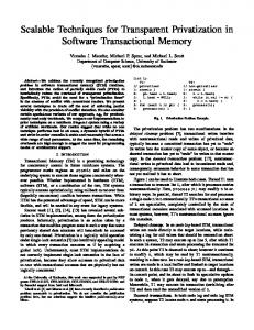
3.1 Basic Idea and Discussion While bottom-up, TSP-based approaches seem to offer the most compressible doc-ID ordering amongst all comparable methods, to achieve this level of compressibility requires significant computational effort. Even though the GNN heuristic simplifies the known NP-Hard TSP problem, approximating a solution in quadratic time, with the millions to billions of documents present in a typical search engine, GNN has difficulty scaling. A solution was proposed in [6] involves a dimensionality reduction through the singular value decomposition (SVD). While offers a substantial improvement in run time, the complexity of this method is still hindered by a quadratic dependency on the size of the corpus, and thus does not scale to typical index sizes. In our approach, we avoid this computational bottleneck by first creating a sparse graph, weeding out the vast majority of the n2 edges used in prior approaches (n = |D|). We then run a GNN approximation to the TSP on this sparse graph, thereby avoiding examining all pairs of nodes. Our goal is to carefully select about k · n edges (where k k other nodes that are likely to contain the k nearest neighbors, using the Locality Sensitive Hashing approach in [15, 13]. We compute for each document t superhashes (here t = 80), where the j-th superhash of each document is computed by selecting l indexes i1 , . . . , il at random from {1, . . . , s}, concatenating the terms selected from the document as the i1 -th, i2 -th, to il -th samples in the previous phase, and hashing the concatenation to a 32-bit integer using MD5 or a similar function. It is important that the same randomly selected indexes i1 , . . . , il are used to select the j-th superhash of every documents. This results in t files F1 to Ft such that Fj contains the the j-th superhash of all documents. The crucial point, analyzed in detail in [13], is that if two documents share the same j-th superhash for some j, their similarity is likely to be above some threshold θ that depends on our choice of s and l. Conversely, if two documents have similarity above θ, and if t is chosen large enough, then it is likely that their j-th superhashes are identical for some j ∈ {1, . . . , t}. Thus, by sorting each file Fj and looking for identical values, we can identify pairs of documents that are likely to be similar. However, for any fixed threshold θ, we may get some nodes with a large number of neighbors with similarity above θ, and some nodes with few or no such neighbors. In order to select about k′ nearest neighbors for each node, we iterate this entire phase several times, starting with a very high similarity threshold θ, and then in each iteration removing nodes that already have enough neighbors and lowering the threshold, until all nodes have enough neighbors. At the end of this phase, we have a long list of candidate nearest neighbor pairs. (3) Filtering: In this phase, we check all the candidate pairs from the previous phase to select the actual k neighbors that we retain for each node. This is done by computing the similarity of each pair using all s samples from the first phase, and selecting the k candidates with highest similarity. (4) TSP Computation: We perform a TSP computation on the sparse subgraph determined in the previous phase, using an appropriate TSP heuristic, for instance GNN, when no outgoing edge is available, we “restart”, mimicking the start heuristic explored in [19], selecting the remaining node with greatest total remaining similarity in the sparse subgraph. Note that this approximation to G, G′ may not even be connected. The ordering
Figure 1: Architecture for LSH-based Dimensionality Reduction for TSP-Based Doc-ID Assignment Algorithms determined by this tour is output and then used to compress the inverted index. This architecture is illustrated in figure 1. We emphasize again that the hashing techniques in phases (1) and (2) are described and analyzed in more detail in [13], and that we reimplemented these phases based on that description. The nearest neighbor candidates are selected based on the Jaccard similarity between documents, but as explained in the next section, it is sometimes beneficial to apply other similarity metrics during the filtering phase, e.g., to try to maximize set intersection rather than Jaccard similarity along the TSP tour. A few comments on efficiency. The first phase requires scanning over and parsing the entire collection, though this could be overlapped with the parsing for index building. Hashing every term s = 100 times is somewhat inefficient, but can be avoided with clever optimizations. The second and third phases require repeated scanning of samples, superhashes, and resulting candidate pairs; the data sizes involved are smaller than the collection but still of significant size (about 5 to 20 GB each as opposed to the 500 GB uncompressed size for the TREC GOV2 data set). However, all steps in these phases scale essentially linearly with collection size (with the caveat that parameters for k, t, and l are adjusted slightly as the collection grows). Moreover, they can be easily and highly efficiently implemented using mapReduce [12] or various I/O-efficient computing paradigms. While the final phase, actual computation of the TSP path, is also the fastest in our setting, this is the only phase that has not been implemented in an I/O efficient paradigm, requiring the entire sparse graph reside in main memory. The min-hashing techniques outlined above provide sufficient compression of this graph such that even the 25 million documents of the TREC GOV2 data set can easily reside in a few GB of main memory. While this data set represents vastly larger set than is evaluated in previous work [19, 6], its size is insignificant in comparison to corpora commonly seen in commercial search engines– data sizes that prevent in-memory computation using even the most powerful servers. While the TSP is very well-studied– literally hundreds of proposed solution schemes exist [10], we were unable to find approximation algorithms designed for external-memory or mapReduce environments. To extend the applicability to the largest document collections, we are currently exploring new TSP algorithms implemented in mapReduce and I/O-efficient computation. Our initial experiments show more scalability and improved path with higher weights compared to GNN used in this paper. We hope to report a full set of results in the final version. In summary, in this section we have shown how to implement the TSP-based approach to the doc-ID assignment problem in an efficient and highly scalable manner, using the well-known hashing techniques in [15, 13]. In the next sections, we show how to refine this approach to optimize the resulting index compression on real data sets and with real index compression technology.
4. CHOOSING EDGE WEIGHTS IN TSP
5. MULTI-GAP OPTIMIZATIONS The TSP approach to document reordering relies on suitable edges weights based on document similarity to find an assignment of docIDs that achieves good compression. However, it is not obvious what is the best measure of document similarity for this case. Previous work has sometimes used the Jaccard measure (the ratio of intersection and union of the two documents) and sometimes used the absolute size of the intersection to determine the edge weight in the resulting TSP problem. We now discuss this issue in more detail and suggest additional weight functions. Intersection size: This measure was previously used in [19, 6], and it also has a simple and meaningful interpretation in the context of the TSP tour. In particular, when we choose some edge of weight w for the tour and thus assign consecutive docIDs to its two endpoints, then this creates w 1-gaps in the index structure. Formally, the maximum TSP tour in a graph with edge weights given by raw intersection size results in an inverted index structure with the largest possible number of 1-gaps. As we show later, using intersection size indeed results in indexes with large numbers of 1-gaps. However, improved compression does not just depend on the number of 1-gaps, as we discuss further below. Jaccard measure: This measure does not have any natural interpretation in terms of gaps, but was previously used in [21, 6]. The Jaccard measure also has two other attractive features in the context of TSP. First, it gives higher weights to documents of similar size. For example, if a small document is properly contained in another larger document, then their Jaccard similarity is very small while their intersection is quite large. While this is not a problem in an optimal solution of the (NP-Complete) TSP problem, many greedy heuristics for TSP appear to suffer by naively choosing edges between documents of very different size. Use of the Jaccard measure discourages use of such edges. Second, the LSH technique from [13] used in our framework works naturally with the Jaccard measure, while scalable nearest-neighbor techniques for other similarity measures are more complicated to implement [15]. Log-Jaccard measure: To explore the space between intersection size and Jaccard, we also tried a hybrid where we divide the intersection size by the logarithm of the size of the union (or some other function), thus discouraging edges between documents of widely different size. Term-weighted intersection: As mentioned before, the resulting compressed index size does not just depend on the number of 1-gaps. In particular, it could be argued that not all 1-gaps are equal: Making a 1000-gap into a 1-gap is more beneficial than making a 2-gap into a 1-gap. This argument is a bit misleading as there is no one-toone correspondence between gaps before and after reordering, but we can restate it in a better way by assuming that docIDs are initially assigned at random. Assume two terms t1 and t2 in the collection, where ft1 and ft2 are the number of postings in the corresponding inverted lists. That means that before the reordering, the average gap was about n/ft1 in the list for t1 and about n/ft2 in the list for t2 (where n is the number of documents), with a geometric distribution around the averages. Thus, if ft1 < ft2 then it could be argued that creating a 1-gap in the list for t1 provides more benefit compared to the case of random assignment than creating a gap in the list for t2 . This leads to a weighted intersection measure where we weigh each term t in the intersection proportional to log(n/ft ), which can also be interpreted as related to the savings obtained from gamma coding a 1-gap rather than an (n/ft )-gap. Implementation of different measures: As mentioned, our LSHbased implementation works naturally with the Jaccard measure. To implement the various other similarity measures, we first use the Jaccardbased LSH method to select the k′ candidates for the nearest neighbors, and then use the filtering phase to rank the candidates according to the actual similarity measure of interest. If k′ is chosen sufficiently larger than k, then this seems to perform quite well.
As discussed, compressed index size does not just depend on the number of 1-gaps. In fact, this motivated our weighted intersection measure in the previous section. We note however that any measure that focuses on 1-gaps, even if suitably weighted, fails to account for the impact of other types of small gaps on index size. A method that increases the number of 1-gaps as well as 2- and 3-gaps might do much better than a method that achieves even more 1-gaps but much fewer other small gaps. Thus, a better approach to document reordering would try to improve the overall distribution of gaps, giving credit for creating 1-gaps as well as other small gaps. However, this collides with a basic assumption in the TSP-based approach, that benefit can be modeled by a weighted edge. A direct TSP formulation can only model 1-gaps! To model larger gaps we have to change the underlying problem formulation so that it considers interactions between documents that are 2, 3, or more positions apart on the TSP tour. Luckily, the greedy TSP algorithm that we implemented can be adjusted to take larger gaps into account. Recall that in this algorithm, we grow a TSP tour by selecting a starting point and then greedily moving to the best neighbor, and from there to a neighbors of that neighbor, and so on. Now assume that we have already chosen a sequence of nodes (sets of terms) d1 , d2 , . . . , di−1 and now have to decide which node to choose as di . For a particular candidate node d, the number of 1-gaps created by choosing d is |d ∩ di−1 |, while the number of 2-gaps is |(d ∩ di−2 ) − di−1 |. More generally, the number of created j-gaps is the number of terms in the intersection of d and di−j that do not occur in any of the documents di−j+1 to di−1 . Thus, we should select the next document on the tour by looking not just at the edge weight, but also at the nodes preceding the last node we selected. To implement this efficiently, we need two additional data structures during the TSP algorithm. We add for each node a compact but sufficiently large sample of its terms. These samples are kept in main memory during the TSP. We found that using a sample of about 10% of the terms, selected by choosing all terms that hash to a value (say) 7 mod 10 for some hash function (such as MD5), works well. This results in a few dozen terms per document which can be compressed to about one byte per term; on the other hand, it is not necessary anymore to store the edge weights in memory as part of the graph as these are now computed online. The second structure is a dictionary that contains for each term that is sampled the index of the last selected document that contained the term. Initially, all entries are set to 0, and when a term t occurs in a newly selected node di during the greedy algorithm, we update its entry to i. Using these structures, the modified algorithm works as follows: Having already selected d1 to di−1 , we select di by iterating over all unvisited neighbors of di−1 , and for each neighbor we iterate over all terms in its sample. For each term, we look at the dictionary to determine the length of the gap that would be created for this term, and compute a suitable weighted total benefit of choosing this document. We then greedily select the neighbor giving the most benefit. We note that this algorithm relies on a basic approach that grows a tour one edge at a time, and could not be easily added to just any algorithm for TSP. Also, note that the filtering step still selects the k nearest neighbors based on a pairwise measure, and we are limited to selecting di from among these neighbors. This leaves us with the problem of modeling the benefit of different gaps. One approach would be to assign a benefit of 1 + log(gavg /j) to any j-gap with j < gavg for a term t, where gavg = n/ft is the average gap in the randomly ordered case as used in the previous section. Thus, a positive benefit is assigned for making a gap smaller than the average gap in the random ordering case, and no benefit is given for any larger gaps. However, this misses an important observation: Reordering of docIDs does not usually result in a reduction in the average d-gap of an inverted list.1 Rather, the goal of reordering is to 1
In fact, if we also count the gap between the last docID in the list and
# of documents # of distinct words # of postings
GOV2 25,205,179 36,759,149 6,797 M
Ireland 10,000,000 18,579,966 2,560 M
Wiki 2,401,798 19,586,472 787 M
Table 1: Basic statistics of our data sets. skew the gap distribution to get many gaps significantly smaller, and a few gaps much larger, than the average. Thus, getting a gap above the average n/ft is actually good, since for every gap above the average, other gaps have to become even smaller! This means that a candidate document should get benefit for containing terms that have recently occurred in another document, and also for not containing terms that have not recently occurred. Or alternatively, we give negative benefit for containing terms that have not recently occurred. This leads us to define the benefit of a j-gap for a term t as 1 + log(gavg /j) for j < gavg and −α · (1 + log(j/gavg )) otherwise, say for α = 0.5.
6.
EXPERIMENTAL EVALUATION
In this section, we evaluate the performance of our scalable TSPbased methods. Note that additional hybrid methods that combine TSP- and sort-based approaches are described and evaluated in Section 7. Throughout this section, we focus on total index size due to docIDs. The impact on the sizes of frequency values and positions will be discussed in later sections.
6.1 Experimental Setup The reductions in index size achievable through reordering depend of course on the properties of the document collection, both in absolute (collections with many similar documents give more gains) and relative terms (sorting-based methods do not work well if URLs or other names are not indicative of content). In our experiments, we use three data sets that are substantially different from each other, in particular:
GOV2 RANDOM SORT TSP-jacc TSP-inter Ireland RANDOM SORT TSP-jacc TSP-inter Wiki RANDOM SORT TSP-jacc TSP-inter
IPC
OPT-PFD
Gamma
% of 1 gaps
6516 2821 2908 2824
6661 3105 3197 3135
8088 3593 3475 3415
7.00% 59.00% 67.90% 68.20%
2467 690 617 610
2502 746 620 614
3820 1020 953 947
8.00% 77.00% 83.80% 84.10%
697 653 594 565
724 714 664 663
1226 1116 1006 984
6.00% 13.00% 28.00% 28.00%
Table 2: Index size in MB and total number of 1-gaps in the index, for the three data sets and four different orderings.
GOV2 RANDOM SORT TSP-jacc TSP-inter Ireland RANDOM SORT TSP-jacc TSP-inter Wiki RANDOM SORT TSP-jacc TSP-inter
IPC
OPT-PFD
Gamma
7.67 3.32 3.42 3.32
7.84 3.66 3.76 3.68
9.52 4.23 4.09 4.02
7.71 2.16 1.92 1.90
7.82 2.33 1.93 1.91
11.94 3.19 2.98 2.96
7.08 6.63 6.03 5.74
7.35 7.25 6.75 6.74
12.45 11.34 10.22 9.82
Table 3: Compression in bits per document ID for the three data • GOV2: The TREC GOV2 collection of 25.2 million pages crawled sets and four document orderings. from the gov domain used in some of the TREC competition tracks. impact of near-duplicates on results in one of our experiments further • Ireland: This is a random sample of 10 million pages taken below. from a crawl of about 100 million pages in the Irish (ie) web 6.2 Comparison of Basic Methods domain provided to us by the Internet Archive. We start by comparing some baseline methods, in particular a ran• Wiki: This is a snapshot of the English version of Wikipedia, dom ordering of docIDs (RANDOM), an ordering according to sorttaken on January 8, 2008, of about 2.4 million wikipedia artiing by URL (SORT), and two methods, TSP-jacc and TSP-inter, based cles. (These are the actual articles, not including other pages on our TSP approach. In particular, in both methods we use our imsuch as discussion, history, or disambiguation pages.) plementation of LSH to determine 400 out-going candidate edges for We note here that the GOV2 collection is very dense in the sense that each node, and then filter these down to 300 out-going edges per node. the gov domain was crawled almost to exhaustion. Thus, for any We then run a greedy Max-TSP algorithm on this graph, where TSPpair of similar pages there is a good chance both pages are in the set, jacc uses the Jaccard measure between two documents as edge weight, and as shown in [22] reductions of about a factor of 2 in index size while TSP-inter uses the raw size of the intersection between the two are achievable for this set. The Ireland data set is a new collection documents. not previously used; by sampling from a larger domain we get a less Tables 2 and 3 show the absolute size of the docID part of the indense set of pages. The Wiki data set is different from the other two verted index, and the number of bits per docID, respectively, for the in that the pages are much more uniform in type and style, and more three data sets. We see that on all data sets, using the raw intersecsimilar to other non-web corpora (e.g., Reuters or WSJ collections). tion size outperforms use of the Jaccard measure. On the Wiki data We also expect less duplication, and less benefit from reordering by set, sorting only gives a minor improvement over random ordering, URL sorting as URLs are probably less meaningful in this case. We while the TSP methods achieve more significant gains, resulting in a plan to look at additional data sets for the final version of this paper. size reduction of up to 19%. For Ireland, sorting does OK, but TSPTable 1 summarizes the basic statistics of the data sets, in particular based methods do much better. On the other hand, for the GOV2 data the number of documents, number of distinct words, and total number set, SORT gets a similar size reduction as TSP-inter (about the same of postings (in millions). In the basic version of these data sets, we did for IPC and OPT-PFD, and less than TSP-inter for Gamma coding). not perform near-duplicate detection to remove pages with different We also see that IPC and OPT-PFD substantially and consistently outURLs that are almost or completely identical. However, we show the perform Gamma coding, with IPC slightly outperforming OPT-PFD. (But note that OPT-PFD has a much higher decompression speed than the end of the collection as a d-gap, then the average d-gap does not either IPC or Gamma [22].) change under any reordering. If we do not count this final gap, then Table 2 also shows the number of 1-gaps (i.e., cases where two conthe average does not change by much for all except very short lists.
Figure 2: Compression in bits per docID on Wiki data as we vary the number of neighbors.
IPC + dups IPC - dups OPT-PFD + dups OPT-PFD - dups Gamma + dups Gamma - dups
RANDOM 6516 4360 6661 4360 8088 6211
SORT 2821 2747 3105 3031 3593 3148
TSP-jacc 2908 2804 3197 3141 3475 3022
TSP-inter 2824 2760 3135 3059 3415 3002
Table 4: Index sizes in MB for GOV2 with and without nearduplicate.
secutive documents in the ordering share a term) for the different ordering methods. TSP-size achieves a significantly higher number of 1-gaps than the others, which is not surprising since the optimal TSP on the complete graph would in fact maximize the total number of 1-gaps. (We believe our simple greedy TSP on the reduced graph is a reasonable approximation.) However, as we see for the case of GOV2, this does not directly imply better compression. TSP-size has many more 1-gaps than SORT, but the resulting compression is about the same. This confirms our conjecture in the previous section, that to minimize size we have to look at more than 1-gaps, and in particular at longer gaps. We now examine how the number of neighbors in the reduced graph impacts performance. In Figure 2, we plot the resulting compression in bits per docID for Wiki as we increase the number of neighbors. For all three compression schemes (IPC, OPT-PFD, Gamma) we see that compression improves with the number of neighbors (as expected), but improvement becomes less significant beyond about 200 to 300 neighbors. In the following, unless stated otherwise, we use 300 neighbors per node, as in our basic experiments above. We note here that a larger number of neighbors increases the time for the TSP-based methods as well as the amount of memory needed during the greedy TSP itself; we explore these issues further below. Next, we consider the impact of near-duplicates (near-dups) on compression. To do this, we used our LSH implementation to detect all near-dups in the three data sets, defined here as pairs of documents with a Jaccard score (ratio of intersection and union) of more than 0.95. (Note that for very short documents, one might argue that this threshold is too strict as it requires two documents to be identical, but such documents contribute only a small part of the postings in the index.) We found that Wiki has less than 0.2% near-dups, while Ireland and GOV2 have 26% and 33% near-dups. But even for the case of GOV2, with more than 8.3 million near-dups out of 25.2 million documents, the benefits of reordering are not just due to near-dups: Removing near-dups from the index under a random ordering results in a size reduction of about 30%, while subsequent reordering of the set without near-dups results in an additional 37% reduction (for IPC, relative to a random ordering without duplicates). Another interesting observation is that for the reordering methods, the size of the index with and without near-dups is very similar – this implies that use of reordering methods effectively neutralizes the
GOV2 SORT TSP-inter TSP-log-ft TSP-log-jacc TSP-gaps Ireland SORT TSP-inter TSP-log-ft TSP-log-jacc TSP-gaps Wiki SORT TSP-inter TSP-log-ft TSP-log-jacc TSP-gaps
IPC
OPT-PFD
Gamma
3.32 3.32 3.47 3.30 3.18
3.66 3.68 3.73 3.68 3.53
4.23 4.02 4.09 4.04 3.96
2.16 1.90 1.91 1.89 1.87
2.33 1.91 1.94 1.91 1.89
3.19 2.96 2.99 2.96 2.91
6.63 5.74 6.09 5.63 5.36
7.25 6.74 6.68 6.31 6.02
11.34 9.82 10.10 9.12 8.83
Table 5: Compressed size for advanced methods in bits per docID.
impact of near-dups on index size, thus allowing us to keep neardups during indexing without index size penalty and then deal with them during query processing (which might sometimes be preferable). Closer inspection of the statistics for near-dups also showed that they are highly skewed and that a significant fraction of the total near-dups in GOV2 and Ireland is due to a small number of documents being near-duplicated many times (rather than due to many documents having one or two near-copies each). We suspect that this is due to the crawler being unable to figure out that (almost) the same content is returned by a site under many different URLs.
6.3 Advanced TSP Methods We now evaluate our various refinements of the basic TSP method. In Table 5 we compare the number of bits per docID of the SORT and TSP-inter methods from above with three additional TSP-based methods described in earlier sections: (i) TSP-log-jacc, which uses as edge weight the size of the intersection divided by the logarithm of the size of the union, (ii) TSP-log-ft, which weighs each term in the intersection of two documents by log(N/ft ) (thus giving higher weights to 1-gaps created in short lists), and (iii) TSP-gaps, which considers not just 1-gaps but also larger gaps as described in Subsection 5. The results are shown in Table 5, where we show the number of bits per docID under IPC, PFD, and Gamma coding. We observe that TSP-log-ft does not seem to give any improvement over using raw intersection, and in fact often does worse. TSP-log-jacc gives decent improvements on Wiki, moderate improvements on GOV2, and only minuscule improvements on Ireland. However, TSP-gaps outperforms all other methods, and achieves improvements, e.g., for IPC, ranging from 2% on Ireland (which may be hard to further improve as it is already less than two bits per docID) to about 8% on Wiki (compared to TSP-inter). Thus, as we conjectured, it is important to model longer gaps, not just 1-gaps, to get the best possible compression. Recall that TSP-gaps is different from the other methods in that it cannot really be modeled as a Max-TSP problem, as the total benefit is not simply a sum of precomputed edge weights but a more complicated expression along the chosen path. However, as discussed in the previous section, we can “graft” this method on top of our simple greedy TSP method that grows a path one edge at a time, by adding suitable data structures and in each step some computation for updating the benefit. A natural question is how much better we could do by using better heuristics for the TSP problem, instead of the simple greedy heuristic used in this and previous work. However, TSP-gaps makes it more difficult to apply other heuristics, as we are restricted to heuristics that grow (one or several) long paths one edge at a time. To test the potential for additional improvements, we experimented with local search strategies that select the next edge to be added to the
GOV2 TSP-gaps TSP-gaps-(5) Ireland TSP-gaps TSP-gaps-(5) Wiki TSP-gaps TSP-gaps-(5) TSP-gaps-(5,5)
IPC
OPT-PFD
Gamma
3.18 3.12
3.53 3.46
3.96 3.90
1.87 1.85
1.89 1.87
2.91 2.87
5.36 5.26 5.25
6.02 5.95 5.93
8.83 8.83 8.81
Table 6: Compression for extended neighborhood search in bits per docID. generating min-hashes generating super-hashes neighbor finding (7 iterations) TSP-jacc TSP-inter TSP-gaps TSP-gaps-(5)
2 hour and 15 minutes 3 hours and 30 minutes 6 hours and 40 minutes 10 minutes 10 minutes 1 hour and 30 minutes 10 hours
Table 7: Time for each step in our TSP-based framework, for GOV2 with 300 neighbors per node.
path by performing a limited search of the neighborhood of the current endpoint. That is, for a depth-d method, we check not just all outgoing edges to select the best one, but for the top-k1 out-going edges, we explore edges at depth 2, and for the top-k2 resulting paths of length 2 we explore one more level, and so on until we have paths of length d. We then add the first edge of the best path to our existing path, and repeat. Thus, a depth-d method is defined by d − 1 parameters k1 to kd−1 , plus a discount factor α that is applied to benefits due to edges further away from the current endpoint, and some threshold value for further pruning of paths (e.g., we might consider only paths with a value at least 80% of the current best path). There are obviously other heuristics one can apply, so this is just a first exploration of the potential for improvements. We note that there is obviously a trade-off with computation time; in a graph with n out-going edges per node, we have to compute the benefit of up to (1 + k1 + . . . kd−1 ) · n instead of n edges. The results are presented in Table 6, where we look at the benefit of a simple depth-2 search (with k1 = 5) over TSP-gaps. We see that the benefits are very limited, with the best improvement of only 2% in index size on the GOV2 and Wiki data set. We also explored the benefit of a deeper search on the Wiki data set and the benefit is very limited.
6.4 Efficiency Issues We now discuss the efficiency of the various methods. We note here that sorting by URL, although not applicable to all data sets, is of course highly efficient as it does not require any access to the text in the documents. Our goal here is not to compete with that speed, but to achieve efficiency that is comparable to that of building a full-text index, and scalability to large data sets. All of our run were performed on a single AMD Opteron 2.3Ghz processor on a machine with 64GB of memory and SATA disks. However, for all experiments at most 8 GB were used, except for the TSP computation in the case of TSPgaps where at most 16 GB were used. Some sample results are shown in Table 7 for the GOV2 collection of 25.2 million pages, our largest data set. In the first step, we create 100 min-hashes per document, while in the second step, 80 32bit super-hashes are created from the min-hashes for each document and for each iteration in the subsequent step (i.e., 560 superhashes per document for the seven iterations). We create a separate file for each
of the 560 super-hashes and then sort each super-hash file using an I/O-efficient merge sort. In the third step, for each node we generate up to 400 candidate nearest-neighbor edges for each node, by performing seven iterations with different threshold values for the LSH computation (using the super-hashes previously created according to the chosen thresholds). Each iteration basically involves a scan over the corresponding 80 super-hash files, and then nodes with more than 400 candidate edges are excluded from subsequent iterations. At the end, the 400 candidates are reranked based on the real weight function (i.e., Jaccard, raw intersection, or log-Jaccard) using the min-hashes, and the top 300 edges for each node are kept. Note that to avoid duplicated candidate edges, we assume that all candidate edges fit in main memory; otherwise we split the nodes into several subset, and perform a scan of superhash scan for each subset. (To use less than 8 GB, we split the nodes into two subsets; otherwise the time for the third step would drop by a factor of 2 while using more memory.) Overall, we note that producing the min-hashes and super-hashes, and then finding and filtering nearest neighbor edges, takes time roughly comparable to that of building a full-text index on such a data set. (The presented running times are reasonably but not completely optimized, so some improvements could be obtained with careful code optimization and tuning of parameters such as the number of neighbors or iterations.) Moreover, we point out that these three steps can be very efficiently and easily ported to a map-reduce environment, or executed in an I/O-efficient manner on a single machine, thus allowing us to scale to much larger data sets. The fourth step is the actual greedy TSP approximation. Our current implementation requires the entire graph reside in main memory– a solution that is inherently non-parrallelizable. We are presently experimenting with new TSP algorithms leveraging mapReduce and I/O efficient techniques to allow arbitrarily large data sets to be processed. Initial experiments are promising, showing improvements in the weight of the TSP solution over the greedy, memory-based TSP approximation used thus far while also scaling to much larger data sets. We will report a full set of experiments in the final version of this paper. As we see, the TSP computation is very fast (around 10 minutes) for precomputed edge weights (e.g., TSP-jacc, TSP-inter, TSP-log-jacc), and somewhat slower (1.5 hours) for the multi-gap approach. TSPgaps also requires more memory to store extra min-hashes (a 10% sample of each document) to compute online the benefits of larger gaps. Once we add an additional search of the neighborhood, the running time quickly increases to about 10 hours even for k1 = 5. Thus, it may be more realistic to avoid this cost and just use TSP-gaps. Overall, for our current GNN, both running time and memory requirements for this step scale roughly linearly with the number of nodes and number of edges per node.
7. HYBRID ALGORITHMS In the previous section, we demonstrated that a TSP-based approach provides significant improvements over the sort-based approach on the Wiki and Ireland data sets and more modest improvements on GOV2, while allowing for a reasonably efficient and scalable implementation. Of course, the sorting-based approach still has advantages in terms of speed, and thus it would be interesting to combine the benefits of the two approaches. In this section, we explore possible hybrid algorithms that use sorting as well as TSP to get better compression and faster computation of the reordering. We start out with a simple extension of the sort-based approach, called SORT+SIZE, where we combine sorting by URL with use of document size. Intuitively, sorting brings similar documents closer together, but probably does not work that well on the local level since very often several groups of similar pages (but different from each other) are mixed in the same site or subdirectory. One simple heuristic to tease such groups apart is to use document size, i.e., the number of words in a document, as an additional feature. In particular, we experimented with the following simple heuristic: We first sort by URL, then in each web site, we split documents into a number of classes ac-
docIDs (IPC) freqs (IPC) total (IPC) docIDs (PFD) freqs (PFD) total (PFD)
RANDOM 6516 1831 8347 6661 2098 8759
SORT 2821 1238 4059 3105 1442 4547
TSP-gaps 2703 1191 3894 3051 1421 4472
Hybrid 2480 1151 3631 2735 1378 4113
Table 9: Total index size in MB including frequency values for GOV2. position (PFD) position (IPC)
Figure 3: Performance of hybrid using both LSH and sort edges on GOV2 under IPC with 300 edges, for varying percentages of LSH edges.
SORT SORT+SIZE TSP-gaps TSP-gaps-(5) Hybrid-50lsh-250sort Hybrid-150lsh-150sort Hybrid-150lsh-150sort+size Hybrid-50lsh-50sort
IPC 3.32 3.23 3.18 3.12 2.96 2.92 2.92 3.02
OPT-PFD 3.66 3.58 3.53 3.46 3.24 3.22 3.22 3.31
Gamma 4.23 4.17 3.96 3.90 3.59 3.57 3.58 3.66
Table 8: Compression in bits per docID for hybrid methods on GOV2. cording to size (usually 5 classes), and then in each class we sort again by URL. (Thus, we first have all the largest pages in the site, then all the moderately large pages, and so on.) As we will show, this simple heuristic already gives interesting improvements in certain cases. It also motivates the search for other heuristics that are only based on simple features such as URL and document size; see for comparison the recent work in [3] on how to detect near-duplicates based only on URLs without using page content. We note that [8] recently and independently proposed to sort all documents by size only; this achieves measurable benefits but does not perform as well as sorting. Next, we consider hybrids between sorting and TSP-based methods. A simple approach would be to first sort by URL, then create for each node edges to its, say, 100 closest neighbors in this ordering, and then run a TSP algorithm on the resulting graph to determine the final ordering. Thus, sorting is used to select edges, and then TSP locally reorders the nodes. We can also combine such sort edges with edges determined via LSH, e.g., 100 edges selected using LSH and 100 neighbor edges from the sorted order. In the following, we experiment with these heuristic. In Figure 3, we look at how to best combine LSH edges and sort edges. Given 300 neighbors, we vary the number of sort edges from 0 to 300, and choose the remaining edges using the LSH method. As we see, this approach achieves significant improvements over our best previous method, decreasing index size by more than 10% in some case over TSP-gaps. We also see that using a roughly equal number of edges from both sets performs best, but that even choosing just 50 LSH edges comes close to optimum. Also, using only sort edges does not perform well at all. We note here that decreasing the number of LSH edges to 50 will significantly reduce the times for the LSH computation (min-hashing, super-hashing, and neighbor finding) reported in the previous section. In Table 8 we present some selected results for the hybrid methods. We see that SORT+SIZE is better than just URL sorting, but not as good as TSP-gaps. We also see that while using 50 LSH edges and 250 sort edges is close to the best result for 300 neighbors, even using just 50 LSH edges and 50 sort edges does better than the best TSP-gaps
RANDOM 3495 3154
SORT 2834 2737
Hybrid 2709 2638
Table 10: Total position index size in MB for a 2-million subset of GOV2. method with 300 neighbors. This is important because using fewer total edges improves both speed and memory consumption for the TSP computation, while using fewer LSH edges improves the efficiency of the various LSH steps. Thus, in practice using 50 sort edges and 50 LSH edges may be a very good choice. However, using sort+size edges instead of sort edges in the hybrid gives no benefits.
8. IMPACT ON QUERY PROCESSING In the preceding sections, we focused on minimizing the total size of the docID part of the inverted index. Of course, one major purpose of minimizing index size is to improve query processing speed, as a smaller index requires less data to be tranferred between disk and memory and between memory and CPU. In this section, we provide a few measurements of the impact of reordering on query processing, using GOV2 and 100000 queries from the TREC Efficiency TASK and Wiki data and 5000 selected queries from AOL which are related to wikipedia. We start out with some numbers for total index size when including frequency values in the index, that is, the number of occurrences of a term in each document. Here, we apply the Most Likely Next (MLN) transformation to frequency values before compression, as proposed in [22]. As we see in Table 9 for the case of GOV2, the methods with the best docID compression also give the best compression for frequency values. Then, we look at the compacts of our new reassignment technique on position compression. In our implementation we treat all documents in the collection as one single consecutive ”big page” and index the position of each term inside this ”big page” as proposed in [11]. Table 10 gives the result for a 2-million subset from GOV2 which have consecutive alphabetic URLs in the total collection. From Table 10 we can see under a better docID assignment the position compression is also improved. Next, we look at the amount of index data per query, that is, the total sizes of the inverted lists associated with the query terms of a typical query. This puts more weight on the most commonly used query terms, and is a measure for the amount of data per query that has to be transferred from disk to main memory in a purely disk-resident index. As we see from Table 11, a better reorderings significantly reduces the amount of index data per query that is needed. In fact, the improvement per query is slightly larger than the improvement in total index size, since more frequently accessed inverted lists appear to benefit more from reordering. State-of-the-art IR query processors cache parts of the inverted in-
size/query
SORT 1.116
TSP-gaps 1.076
Hybrid 0.98
Table 11: Size of inverted lists per query for docID in MB, for GOV2 using IPC.
in initial runs, and the use of additional data sets, in particular the Reuters and WSJ collections and one other broad-based web corpus. There are a number of open questions for future work. It would be interesting to look at other reordering heuristics that only use meta data such as URLs, mime type, and document size, motivated by work in [3]. Since document reordering is known to lead to more skips in the inverted lists during query processing [22], one could try to directly optimize the docID ordering for this objective, leading to faster query processing. Finally, a major limitation of document reordering techniques is that they are often not applicable in the presence of early termination techniques for query processing that assume a particular ordering of the index structures. It would be interesting to explore trade-offs between and possible combinations of early termination and document reordering techniques.
10. REFERENCES [1] V. Anh and A. Moffat. Inverted index compression using word-aligned binary Figure 4: Amount of index data in MB per query that has to be fetched from disk, for cache sizes ranging from 0 to 640 MB. Random Sort TSP-gaps
query processing time(ms/query) 0.274 0.256 0.192
decoded postings(k/query) 91264 81920 60416
Table 12: Query processing performance on Wikipedia dex in main memory in order to reduce disk accesses and thus speed up processing. We now look at how disk tranfers are reduced by using a better document ordering. It is important to realize that the reduction in disk accesses is not linear in either the total or per-query index size, but usually much larger since a higher percentage of the smaller index will fit into cache, thus in turn increasing the cache hit rate. In Figure 4 we see that both TSP-gaps and the hybrid method achieve fairly significant improvements over the sort-based ordering for a range of cache sizes from 0 to 640 MB, resulting in up to 24% reduction in disk transfers. Finally, it was shown in [22] that reordering also significantly reduces the CPU costs of intersecting inverted lists in main memory, as it results in larger skips within the lists. As we see from Table 12, a better reorderings can reduce the amount of time on query processing by up to 25% compared with sorting. We note that all our algorithms here only explicitly try to optimize docID compression, and not frequency and position compression or query processing. Optimizing directly for these measure is an open problem for future research.
9.
DISCUSSION AND CONCLUSIONS
In this paper, we proposed and evaluated new algorithms for docID assignment that attempt to minimize index size. In particular, we described a framework for scaling the TSP-based approach, shown to perform well in previous work but expensive to compute, to much larger data sets by using Locally Sensitive Hashing (LSH). Within this approach, we experimented with different objective functions, search heuristics, and hybrids, and showed that the TSP approach can significantly outperform sorting by URL, the best previously known approach that scales to such large data sets. Overall, the main lessons from this work are that the TSP approach can be applied to sets of tens of millions of pages, that the TSP-gaps approach in particular appears to give a reasonable balance between computational cost and index size, and that in some cases selecting candidates edges using both sorting and LSH results in additional improvements over TSP-gaps. There are still a few tasks in our experimental evaluation that we are currently working on. This includes the new TSP algorithm which can be implemented using mapReduce or I/O efficient computation, which already gives improved performance
codes. Information Retrieval, 8(1):151–166, Jan. 2005. [2] A. Bagchi, A. Bhargava, and T. Suel. Approximate maximum weighted branchings. In Information Processing Letters, volume 99, 2006. [3] E. Baykan, M. R. Henzinger, L. Marian, and I. Weber. Purely url-based topic classification. In 18th International World Wide Web Conference (WWW2009), April 2009. [4] R. Blanco and A. Barreiro. Characterization of a simple case of the reassignment of document identifiers as a pattern sequencing problem. In Proc. of the 28th annual int. ACM SIGIR conference on Research and development in information retrieval, pages 587–588, 2005. [5] R. Blanco and A. Barreiro. Document identifier reassignment through dimensionality reduction. In Proc. of the 27th European Conf. on Information Retrieval, pages 375–387, 2005. [6] R. Blanco and A. Barreiro. Tsp and cluster-based solutions to the reassignment of document identifiers. Inf. Retr., 9(4):499–517, 2006. [7] D. Blandford and G. Blelloch. Index compression through document reordering. In Proc. of the Data Compression Conference, pages 342–351, 2002. [8] B. Brewington and G. Cybenko. Keeping up with the changing web. IEEE Computer, 33(5), May 2000. [9] A. Broder, M. Charikar, A. Frieze, and M. Mitzenmacher. Min-wise independent permutations. In Proc. of the 30th Annual ACM Symp. on Theory of Computing, pages 327–336, May 23–26 1998. [10] V. C. David L. Applegate, Robert E. Bixby and W. J. Cook. The traveling salesman problem: A computational study, 2006. [11] J. Dean. Challenges in building large-scale information retrieval systems. In Second ACM International Conference on Web Search and Data Mining (WSDM2009), April 2009. [12] J. Dean and S. Ghemawat. Mapreduce: Simplified data processing on large clusters. 6th symposium on operating system design and implementation. pages 137–150, 2004. [13] T. Haveliwala, A. Gionis, and P. Indyk. Scalable techniques for clustering the web. In Proc. of the WebDB Workshop, Dallas, TX, May 2000. [14] S. Heman. Super-scalar database compression between RAM and CPU-cache. MS Thesis, Centrum voor Wiskunde en Informatica, Amsterdam, Netherlands, July 2005. [15] P. Indyk and R. Motwani. Approximate nearest neighbors: Towards removing the curse of dimensionality. In Proc. of the 30th ACM Symp. on Theory of Computing, pages 604–612, May 1998. [16] A. Moffat and L. Stuiver. Binary interpolative coding for effective index compression. Information Retrieval, 3(1):25–47, 2000. [17] Z. Ouyang, N. Memon, T. Suel, and D. Trendafilov. Cluster-based delta compression of a collection of files. In Third Int. Conf. on Web Information Systems Engineering, December 2002. [18] F. Scholer, H. Williams, J. Yiannis, and J. Zobel. Compression of inverted indexes for fast query evaluation. In Proc. of the 25th Annual SIGIR Conf. on Research and Development in Information Retrieval, pages 222–229, Aug. 2002. [19] W. Shieh, T. Chen, J. Shann, and C. Chung. Inverted file compression through document identifier reassignment. Inf. Processing and Management, 39(1):117–131, 2003. [20] F. Silvestri. Sorting out the document identifier assignment problem. In Proc. of 29th European Conf. on Information Retrieval, pages 101–112, 2007. [21] F. Silvestri, S. Orlando, and R. Perego. Assigning identifiers to documents to enhance the clustering property of fulltext indexes. In Proc. of the 27th Annual Int. ACM SIGIR Conference on Research and Development in Information Retrieval, pages 305–312, 2004. [22] H. Yan, S. Ding, and T. Suel. Inverted index compression and query processing with optimized document ordering. In 18th International World Wide Web Conference (WWW2009), April 2009. [23] J. Zhang, X. Long, and T. Suel. Performance of compressed inverted list caching in search engines. In Proc. of the 17th Int. World Wide Web Conference, April 2008. [24] J. Zobel and A. Moffat. Inverted files for text search engines. ACM Computing Surveys, 38(2), 2006. [25] M. Zukowski, S. Heman, N. Nes, and P. Boncz. Super-scalar RAM-CPU cache compression. In Proc. of the Int. Conf. on Data Engineering, 2006.