Efficient Binary Field Arithmetic and Applications to Curve-based ...

Efficient Binary Field Arithmetic and Applications to Curve-based Cryptography Diego F. Aranha Department of Computer Science University of Bras´ılia

CHES 2012 Tutorial

Diego F. Aranha

Efficient Binary Field Arithmetic

Part I: RELIC

Diego F. Aranha


Numbers

RELIC is an Efficient LIbrary for Cryptography (http://code.google.com/p/relic-toolkit): Research framework Licensed as free software (LGPL)

Relic

toolkit

11 source code releases 78,000 lines of code 1300 visitors from 74 countries 1500 downloads

Diego F. Aranha


Introduction

Limitations of other libraries: Restricted portability Uninteresting licensing model Emphasis on standards and commercial algorithms Why a new criptographic library? Organization oriented for portability Complete control of licensing model Code sharing and reproducibility of results Focus on research

Diego F. Aranha


Relic

toolkit

Organization Basic organization: Meta-library Compile-time configuration Inspired on GNU Multiple Precision Arithmetic Library (GMP) Protocols

Arithmetic backend

Diego F. Aranha


Breakdown Arithmetic backend: Architecture-dependent Rigid interface with upper layers Generic modules available in C and with GMP support 21 functions for multiple precision integer arithmetic, 26 functions for binary fields, 32 functions for prime fields Why this organization? It is currently possible to obtain competitive timings with the same library in an 8-bit processor with 4KB of RAM and an 8-core Intel desktop processor.

Diego F. Aranha


Breakdown Binary field arithmetic: Field size specified on compile time 3 different strategies for squaring, 5 for multiplication, 2 for square root extraction, 2 for half-trace and 6 for inversion Modular reduction by trinomials and pentanomials Binary curve arithmetic: Supersingular, Koblitz and ordinary (standardized or not) Affine, projective and mixed coordinate systems 4 different strategies for random point scalar multiplication, 6 for fixed point and 4 for multiple point Symmetric pairings over genus-1 or genus-2 curves

Diego F. Aranha


Breakdown Miscellaneous: Support for words of 8, 16, 32 and 64 bits Static, stack, automatic and dynamic memory allocators Helper macros for testing and benchmarking Support for debugging, profiling, tracing and multithreading Abundant Doxygen documentation Deactivation of modules and automatic elimination of algorithms to reduce code size Standard PRNG with configurable seed source Support for FreeBSD, Linux, Mac OS X, Windows Management of configuration and build system with CMake Open collaboration with academia and industry

Diego F. Aranha


Part II: Binary fields

Diego F. Aranha


Introduction

A finite field Fpm consists of all polynomials with coefficients in Zp , prime p, modulo an irreducible degree-m polynomial f (z). Prime p is the characteristic of the field and m is the extension degree. A binary field F2m is the special case p = 2 and is formed by polynomials with binary coefficients.

Diego F. Aranha


Introduction

Example: Field F28 Irreducible polynomial: f (z) = z 8 + z 4 + z 3 + z + 1 = 1 0001 1011 Representation: a(z) = z 7 + z 3 + 1 = 1000 1001 = 0x89 b(z) = z 6 + z 5 + z 2 = 0110 0100 = 0x64 Addition: a(z) + b(z) = z 7 + z 6 + z 5 + z 3 + z 2 + 1 = 1110 1101 = 0xED Note: a(z) + a(z) = 2 · a(z) = 0, ∀a ∈ F2m

Diego F. Aranha


Introduction Example: Field F28 Irreducible polynomial: f (z) = z 8 + z 4 + z 3 + z + 1 = 1 0001 1011 Representation: a(z) = z 7 + z 3 + 1 = 1000 1001 = 0x89 b(z) = z 6 + z 5 + z 2 = 0110 0100 = 0x64 Multiplication: a(z) × b(z) = z 13 + z 12 + z 8 + z 6 + z 2 mod f (z) = z 7 + z 5 + z 4 + z 3 + z 2 + 1 = 0xBD Multiplication by z: z × b(z) = z 7 + z 6 + z 3 = 1100 1000 = 0xC8 = b 1

Diego F. Aranha


Introduction

Binary fields (F2m ) are omnipresent in Cryptography: Efficient Curve-based Cryptography (ECC, PBC) Post-quantum Cryptography Block ciphers Many algorithms/optimizations already described in the literature: Is it possible to unify the fastest ones in a simple formulation? Can such a formulation reflect the state-of-the-art and provide new ideas?

Diego F. Aranha


Objective

Contributions Formulation of state-of-the-art binary field arithmetic using vector instructions New strategy for the implementation of multiplication Time-memory trade-offs to compensate for native multiplier Experimental results

Diego F. Aranha


Arsenal Intel Core architecture: 128-bit Streaming SIMD Extensions instructions (65/45 nm) Super shuffle engine introduced in 45 nm series Carry-less multiplier introduced in Nehalem family 256-bit Advanced Vector Extensions instructions (32 nm) Relevant vector instructions: Instruction MOVDQA PSLLQ, PSRLQ PXOR,PAND,POR PUNPCKLBW/HBW PSLLDQ,PSRLDQ PSHUFB PALIGNR PCLMULQDQ

Description Memory load/store 64-bit bitwise shifts Bitwise XOR,AND,OR Byte interleaving 128-bit bytewise shift Byte shuffling Memory alignment Carry-less multiplication Diego F. Aranha

Cost 3/2 1 1 3 2 (1) 3 (1) 2 (1) 10 (8)

Mnemonic ← -8 , -8 ⊕, ∧, ∨ interlo/hi 8 , 8 shuffle,lookup C ⊗


New SSSE3 instructions PSHUFB instruction ( mm shuffle epi8):

Real power: We can implement in parallel any function:

Diego F. Aranha


New SSSE3 instructions Example: Bit manipulation

Diego F. Aranha


New SSSE3 instructions

PALIGNR instruction ( mm alignr epi8):

Diego F. Aranha


Binary field F2m

Irreducible polynomial: f (z) (trinomial or pentanomial)

Polynomial basis: a(z) ∈ F2m =

m−1 X

ai z i .

i=0

Software representation: vector of n = dm/64e words (even). Graphical representation:

Diego F. Aranha


Data types

# if WORD == 8 typedef uint8_t dig_t ; # elif WORD == 16 typedef uint16_t dig_t ; # elif WORD == 32 typedef uint32_t dig_t ; # elif WORD == 64 typedef uint64_t dig_t ; # endif typedef __m128i vec_t ;

Diego F. Aranha


Useful macros

# define # define # define # define # define # define # define # define # define # define # define # define

LOAD STORE PSHUFB XOR AND SHL SHR SHL8 SHR8 UNPACKLO UNPACKHI CLMUL

_mm_load_si128 _mm_store_si128 _mm_shuffle_epi8 _mm_xor_si128 _mm_and_si128 _mm_slli_epi64 _mm_srli_epi64 _mm_slli_si128 _mm_srli_si128 _mm_unpacklo _epi8 _mm_unpackhi _epi8 _m m_ clmul epi 64_ si12 8

Diego F. Aranha


Proposed representation

To employ 4-bit granular arithmetic, convert to split form: X X aL = ai z i , aH = ai z i−4 , 0≤i 4 Easy to convert back: a(z) = aH (z)z 4 + aL (z).

Diego F. Aranha


Addition/subtraction in F2m c(z) = a(z) + b(z) =

m−1 X

(ai ⊕ bi )z i

i=0

AA BB

n-1

n-1

...

A9 A8 A7 A6 A5 A4 A3 A2 A1 A0

...

B9 B8 B7 B6 B5 B4 B3 B2 B1 B0

+ + + + + + + + + + + +

CC

n-1

...

C9 C8 C7 C6 C5 C4 C3 C2 C1 C0

Guidelines: Use XOR instruction with largest operand size. Verify impact of higher throughput. Diego F. Aranha


Addition/subtraction in F2m

void fb_addn_low ( dig_t *c , int i ; for ( i = 0; i < FB_DIGS ; vec_t t0 = LOAD (( vec_t vec_t t1 = LOAD (( vec_t t0 = XOR ( t0 , t1 ); STORE (( vec_t *) c , t0 ); } }

Diego F. Aranha

dig_t *a , dig_t * b ) { i += 2 , c += 2 , a += 2 , b += 2) { *) a ); *) b );


Squaring in F2m

a(z) =

m X

ai z i = am−1 + · · · + a2 z 2 + a1 z + a0

i=0

a(z)2 =

m−1 X

ai z 2i = am−1 z 2m−2 + · · · + a2 z 4 + a1 z 2 + a0

i=0

Example: a(z) = (am−1 , am−2 , . . . , a2 , a1 , a0 ) a(z)2 = (am−1 , 0, am−2 , 0, . . . , 0, a2 , 0, a1 , 0, a0 )

Diego F. Aranha


Squaring in F2m Since squaring is a linear operation: a(z)2 = aH (z)2 · z 8 + aL (z)2 . We can compute aL (z)2 and aH (z)2 with a lookup table. For u = (u3 , u2 , u1 , u0 ), use table(u) = (0, u3 , 0, u2 , 0, u1 , 0, u0 ):

Diego F. Aranha


Proposed squaring in F2m Ai AL

AH

table

01010101

...

00010001 00010000

00000101 00000100 00000001 00000000

lookup

lookup

AH

AL interhi, interlo

T 2i+1

T 2i

a(z)2 = aL (z)2 + aH (z)2 · z 8 . Diego F. Aranha


Squaring in F2m Algorithm 1 Proposed optimization for squaring in F2m . Input: a(z) = a[0..n − 1]. Output: c(z) = c[0..n − 1] = a(z)2 mod f (z). 1: Store in table the squares u(z)2 of all 4-bit polynomials u(z). 2: table ← (0x5554515045444140,0x1514111005040100) 3: mask ← (0x0F0F0F0F0F0F0F0F,0x0F0F0F0F0F0F0F0F) 4: for i ← 0 to n2 − 1 do 5: a0 ←load(a[2i]) 6: Convert to split representation. 7: aL ← a0 ∧ mask 8: aH ← a0 -8 4, aH ← aH ∧ mask 9: Perform parallel table lookups. 10: aL ←lookup(table, aL ), aH ←lookup(table, aH ) 11: Simulate addition with 8-bit offset. 12: t[2i] ←interlo(aL , aH ) 13: t[2i + 1] ←interhi(aL , aH ) 14: end for 15: return c = t mod f (z) Diego F. Aranha


Squaring in F2m void fb_sqrm_low ( dig_t *c , dig_t * a ) { vec_t t0 , t1 , t2 , t3 , mask ; t0 = _mm_set_epi32 (0 x55545150 , 0 x45444140 , 0 x15141110 , 0 x05040100 ); mask = _mm_set_epi32 (0 x0F0F0F0F , 0 x0F0F0F0F , 0 x0F0F0F0F , 0 x0F0F0F0F ); for ( int i = 0; i < FB_DIGS ; i += 2) { t1 = LOAD (( vec_t *)( a + i )); t2 = AND ( t1 , mask ); t2 = PSHUFB ( t0 , t2 ); t3 = SHR ( t1 , 4); t3 = AND ( t3 , mask ); t3 = PSHUFB ( t0 , t3 ); t1 = UNPACKLO ( t2 , t3 ); t2 = UNPACKHI ( t2 , t3 ); STORE (( vec_t *)( c + 2* i ) , t1 ); STORE (( vec_t *)( c + 2*( i + 1)) , t2 ); } REDUCE (c , c ); } Diego F. Aranha


Square root extraction in F2m Algorithm by Fong et al.: √

a = a2

m−1

=

m−1 X

ai z i

2m −1

i=0

=

=

m−1 X

ai z 2

m −1

i

i=0

i

X

ai z 2 +

i even

√

= aeven +

√ X i−1 z ai z 2 i odd

z · aodd

Since square-root is also a linear operation: q p a(z) = aH (z)z 4 + aL (z) p p = aH (z)z 2 + aL (z) √ = z · (aLodd (z) + aHodd (z)z 2 ) + aLeven (z) + aHeven (z)z 2 √ Note: Multiplication by z ideally requires shifted additions only. √ If not possible, precompute product by z. Diego F. Aranha


Proposed square root in F2m Ai shuffle

AL table

AH 00110011

...

00000001 00000000

11001100

...

00000100 00000000

table · z²

lookup

lookup

AH

AL

AL

AH

A even

p

a(z) =

√

Aodd

z · (aLodd (z) + aHodd (z)z 2 ) + aLeven (z) + aHeven (z)z 2 Diego F. Aranha


Multiplication in F2m

Three strategies: 1

López-Dahab comb method

2

Shuffle-based multiplication

3

Native multiplication

Diego F. Aranha


López-Dahab multiplication in F2m We can compute u · b(z) using shifts and additions.

If a(z) is divided into 4-bit polynomials, compute a(z) · b(z) by:

Diego F. Aranha


López-Dahab multiplication in F2m

If the multiplier is represented in split form: a(z) · b(z) = b(z) · (aH (z)z 4 + aL (z)) = b(z)z 4 aH (z) + b(z)aL (z)

This is a well-known technique for removing expensive 4-bit shifts! Note: The core operation is accumulating u × dense b(z).

Diego F. Aranha


López-Dahab multiplication in F2m Algorithm 2 LD multiplication implemented with n 128-bit registers. Input: a(z) = a[0..n − 1], b(z) = b[0..n − 1]. Output: c(z) = c[0..n − 1]. Note: mi denotes the vector of n2 128-bit registers (r(i−1+n/2) , . . . , ri ). 1: Compute T0 (u) = u(z) · b(z), T1 (u) = u(z) · (b(z)z 4 ) for all u(z) of degree < 4. 2: (rn−1 . . . , r0 ) ← 0 3: for k ← 56 downto 0 by 8 do 4: for j ← 1 to n − 1 by 2 do 5: Let u = (u3 , u2 , u1 , u0 ), where ut is bit (k + t) of a[j]. 6: Let v = (v3 , v2 , v1 , v0 ), where vt is bit (k + t + 4) of a[j]. 7: m(j−1)/2 ← m(j−1)/2 ⊕ T0 (u), m(j−1)/2 ← m(j−1)/2 ⊕ T1 (v ) 8: end for 9: (rn−1 . . . , r0 ) ← (rn−1 . . . , r0 ) C 8 10: end for 11: for k ← 56 downto 0 by 8 do 12: for j ← 0 to n − 2 by 2 do 13: Let u = (u3 , u2 , u1 , u0 ), where ut is bit (k + t) of a[j]. 14: Let v = (v3 , v2 , v1 , v0 ), where vt is bit (k + t + 4) of a[j]. 15: mj/2 ← mj/2 ⊕ T0 (u), mj/2 ← mj/2 ⊕ T1 (v ) 16: end for 17: if k > 0 then (rn−1 . . . , r0 ) ← (rn−1 . . . , r0 ) C 8 18: end for 19: return c = (rn−1 . . . , r0 ) mod f (z) Diego F. Aranha


Shuffle-based multiplication in F2m

If both multiplicand and multiplier are represented in split form: a(z) · b(z) = (bH (z)z 4 + bL (z)) · (aH (z)z 4 + aL (z))

Using Karatsuba formula, we can reduce it to 3 multiplications: a(z)·b(z) = aH bH z 8 +[(aH + aL )(bH + bL ) + aH bH + aL bL ] z 4 +aL bL Note: The core operation is accumulating u × sparse bL,H (z). x

B

n-1

...

B 9 B 8 B 7 B6 B 5 B 4 B 3 B 2 B 1 B 0

Diego F. Aranha


Shuffle-based multiplication in F2m Algorithm 3 Multiplication in split form. Input: Operands a, b in split representation. Output: Result a · b stored in registers (rn−1 . . . , r0 ). 1: table stores all products of 4-bit × 4-bit polynomials. 2: (rn−1 . . . , r0 ) ← 0 3: for k ← 56 downto 0 by 8 do 4: for j ← 1 to n − 1 by 2 do 5: Let u = (u3 , u2 , u1 , u0 ), where ut is bit (k + t) of a[j]. 6: for i ← 0 to n2 − 1 do ri ← ri ⊕ shuffle(table[u], b[i]) 7: end for 8: (rn−1 . . . , r0 ) ← (rn−1 . . . , r0 ) C 8 9: end for 10: for k ← 56 downto 0 by 8 do 11: for j ← 0 to n − 2 by 2 do 12: Let u = (u3 , u2 , u1 , u0 ), where ut is bit (k + t) of a[j]. 13: for i ← 0 to n2 − 1 do ri ← ri ⊕ shuffle(table[u], b[i]) 14: end for 15: if k > 0 then (rn−1 . . . , r0 ) ← (rn−1 . . . , r0 ) C 8 16: end for Diego F. Aranha


Native multiplication

Two organizations: 1

128-bit granularity: Reduce number of required registers Use Karatsuba for each 128 × 128-bit multiplication Use maximum number of Karatsuba levels for n2 digits

2

64-bit granularity: Interleave storage to reduce additions and number of registers Use the formula with the lower number of multiplications

Diego F. Aranha


Native multiplication Algorithm 4 Proposed implementation for multiplication in F2283 . Input: a(z) = a[0..4], b(z) = b[0..4]. Output: c(z) = c[0..4] = a(z) · b(z). Note: Pairs ai , bi , ci , mi of 64-bit words represent vector registers. 1: for i ← 0 to 4 do ci ← (a[i], b[i]) 2: c5 ← c0 ⊕ c1 , c6 ← c0 ⊕ c2 , c7 ← c2 ⊕ c4 , c8 ← c3 ⊕ c4 3: c9 ← c3 ⊕ c6 , c10 ← c1 ⊕ c7 , c11 ← c5 ⊕ c8 , c12 ← c2 ⊕ c11 4: for i ← 0 to 12 do mi ← ci [0] ⊗ ci [1] 5: c0 ← m0 , c8 ← m4 6: c1 ← c0 ⊕ m1 , c2 ← c1 ⊕ m6 7: c1 ← c1 ⊕ m5 , c2 ← c2 ⊕ m2 8: c7 ← c8 ⊕ m3 , c6 ← c7 ⊕ m7 9: c7 ← c7 ⊕ m8 , c6 ← c6 ⊕ m2 10: c5 ← m11 ⊕ m12 , c3 ← c5 ⊕ m9 11: c3 ← c3 ⊕ c0 ⊕ c10 12: c4 ← c1 ⊕ c7 ⊕ m9 ⊕ m10 ⊕ m12 13: c5 ← c5 ⊕ c2 ⊕ c8 ⊕ m10 14: c9 ← c7 8 64 15: (c7 , c5 , c3 , c1 ) ← (c7 , c5 , c3 , c1 ) C 8 16: c0 ← c0 ⊕ c1 , c1 ← c2 ⊕ c3 , c2 ← c4 ⊕ c5 17: c3 ← c6 ⊕ c7 , c4 ← c8 ⊕ c9 18: return c = (c4 , c3 , c2 , c1 , c0 ) mod f (z) Diego F. Aranha


Comparison López-Dahab multiplication: Explores highest-granularity XOR operation Consumes memory space proportional to field size Shuffle-based multiplication: Relies on sparser core operation Consumes constant memory space (apart from Karatsuba) Depends on constants stored in memory Native multiplication: Faster and with constant memory consumption. No widespread support.

Diego F. Aranha


Modular reduction

We need to reduce squaring/multiplication results in F2m modulo f (z) = z m + r (z). We can process multiple bits at a time based on the observation: c(z) = c2m−2 z 2m−2 + · · · + cm z m + cm−1 z m−1 + . . . c1 z + c0 = (c2m−2 z m−2 + · · · + cm )r (z) + cm−1 z m−1 + . . . c1 z + c0 .

Important: We need to multiply by r (z).

Diego F. Aranha


Modular reduction

Requires heavy shifting, so split representation does not help. Guidelines: If f (z) is a trinomial, implement with vector digits If f (z) is a pentanomial, process pairs of digits in parallel or 64-bit mode Write f (z) in a format that minimizes shifting: f (z) = z 283 + z 12 + z 7 + z 5 + 1 = z 283 + (z 7 + 1)(z 5 + 1) Accumulate writes into registers before writing to memory Reduce squaring/multiplication results in registers

Diego F. Aranha


Modular reduction (64-bit mode) Algorithm 5 Fast modular reduction by f (z) = z 1223 + z 255 + 1. Input: c(z) = c[0..2n − 1]. Output: c(z) mod f (z) = c[0..n − 1]. 1: for i ← 2n − 1 downto n do 2: t ← c[i] 3: c[i − 15] ← c[i − 15] ⊕ (t 8) 4: c[i − 16] ← c[i − 16] ⊕ (t 56) 5: c[i − 19] ← c[i − 19] ⊕ (t 7) 6: c[i − 20] ← c[i − 20] ⊕ (t 57) 7: end for 8: t ← c[19] 7, c[0] ← c[0] ⊕ t, t ← t 7 9: c[3] ← c[3] ⊕ (t 56) 10: c[4] ← c[4] ⊕ (t 8) 11: c[19] ← (c[19] ⊕ t) ∧ 0x7F 12: return c

Diego F. Aranha


Modular reduction (128-bit mode) Algorithm 6 Proposed fast reduction by f (z) = z 1223 + z 255 + 1. Input: t(z) = t[0..n − 1] (vector of 128-bit elements). Output: c(z) mod f (z) = c[0..n − 1]. Note: The accumulate function R(r3 , r2 , r1 , r0 , t) executes: s ← t -8 7, r3 ← t -8 57 r3 ← r3 ⊕ (s 8 64) r2 ← r2 ⊕ (s 8 64) r1 ← r1 ⊕ (t 8 56) r0 ← r0 ⊕ (t 8 72) 1: r0 , r1 , r2 , r3 ← 0 2: for i ← 19 downto 15 by 4 do 3: R(r3 , r2 , r1 , r0 , t[i]), t[i − 7] ← t[i − 7] ⊕ r0 4: R(r0 , r3 , r2 , r1 , t[i − 1]), t[i − 8] ← t[i − 8] ⊕ r1 5: R(r1 , r0 , r3 , r2 , t[i − 2]), t[i − 9] ← t[i − 9] ⊕ r2 6: R(r2 , r1 , r0 , r3 , t[i − 3]), t[i − 10] ← t[i − 10] ⊕ r3 7: end for 8: R(r3 , r2 , r1 , r0 , t[11]), t[4] ← t[4] ⊕ r0 9: R(r0 , r3 , r2 , r1 , t[10]), t[3] ← t[3] ⊕ r1 10: t[2] ← t[2] ⊕ r2 , t[1] ← t[1] ⊕ r3 , t[0] ← t[0] ⊕ r0 11: r0 ← m[9] 8 64, r0 ← r0 -8 7, t[0] ← t[0] ⊕ r0 12: r1 ← r0 8 64, r1 ← r1 -8 63, t[1] ← t[1] ⊕ r1 13: r1 ← r0 -8 1, t[2] ← t[2] ⊕ r1 14: for i ← 0 to 9 do c[2i] ← store(t[i]), c[19] ← c[19] ∧ 0x7F 15: return c Diego F. Aranha


Modular reduction (128-bit mode) Algorithm 7 Proposed fast reduction by f (z) = z 283 + (z 7 + 1)(z 5 + 1). Input: Double-precision polynomial stored into 128-bit registers c = (c4 , c3 , c2 , c1 , c0 ). Output: Field element c mod f (z) stored into 128-bit registers (c2 , c1 , c0 ). 1: t2 ← c2 , t0 ← (c3 , c2 ) B 64, t1 ← (c4 , c3 ) B 64 2: c4 ← c4 -8 27, c3 ← c3 -8 27, c3 ← c3 ⊕ (t1 -8 37) 3: c2 ← c2 -8 27, c2 ← c2 ⊕ (t0 -8 37) 4: t0 ← (c4 , c3 ) B 120, c4 ← c4 ⊕ (t0 -8 1) 5: t1 ← (c3 , c2 ) B 64, c3 ← c3 ⊕ (c3 -8 7) ⊕ (t1 -8 57) 6: t0 ← c2 8 64, c2 ← c2 ⊕ (c2 -8 7) ⊕ (t0 -8 57) 7: t0 ← (c4 , c3 ) B 120, c4 ← c4 ⊕ (t0 -8 3) 8: t1 ← (c3 , c2 ) B 64, c3 ← c3 ⊕ (c3 -8 5) ⊕ (t1 -8 59) 9: t0 ← c2 8 64, c2 ← c2 ⊕ (c2 -8 5) ⊕ (t0 -8 59) 10: c0 ← c0 ⊕ c2 , c1 ← c1 ⊕ c3 , c2 ← t2 ⊕ c4 11: t0 ← c4 -8 27 12: t1 ← t0 ⊕ (t0 -8 5) 13: t0 ← t1 ⊕ (t1 -8 7) 14: c0 ← c0 ⊕ t0 , c2 ← c2 ∧ (0x0000000000000000,0x0000000007FFFFFF) 15: return c = (c2 , c1 , c0 )

Diego F. Aranha


Half-trace We want to compute H(c) =

P(m−1)/2 i=0

2i

c2 .

Important: For even i, H(z i ) = H(z i/2 ) + z i/2 + Tr (z i ). Algorithm 8 Solve x 2 + x = c P i m Input: c = m−1 i=0 ci z ∈ F2 where m is odd and Tr (c) = 0 Output: solution s of x 2 + x = c.

1: 2: 3: 4: 5: 6: 7: 8:

Compute H(l0 z 8i+1 + l1 z 8i+3 + l2 z 8i+5 + l3 z 8i+7 ) for 0 ≤ i ≤ b m−3 c and lj ∈ F2 . 8 s←0 for i = (m − 1)/2 downto 1 do if c2i = 1 then c ← c + zi , s ← s + zi end if end for P return s + i∈I c8i+1 H(z 8i+1 ) + c8i+3 H(z 8i+3 ) + c8i+5 H(z 8i+5 ) + c8i+7 H(z 8i+7 )

Diego F. Aranha


Multi-squaring [Bos et al.]

Precompute a table T of 16d m4 e field elements such that T [j, i0 + 2i1 + 4i2 + 8i3 ] = (i0 z 4j + i1 z 4j+1 + i2 z 4j+2 + i3 z 4j+3 )2 k

Then we can compute a2 as: m

k

a2 =

d4e X

T [j, ba/24j c mod 24 ].

j=0

Diego F. Aranha


k

Inversion

Guidelines: If memory is not available, implement Extended Euclidean Algorithm in 64-bit mode. If memory is available, implement Itoh-Tsuji with precomputed 2i powers: m−1 −1)2

a−1 = a(2

Diego F. Aranha


Inversion Algorithm 9 Inversion in F2m using EEA. P i Input: a = m−1 i=0 ai z ∈ F2m Output: a−1 mod f . 1: u ← a, v ← f 2: g1 ← 1, g2 ← 0 3: while u 6= 1 do 4: j ← deg (u) − deg (v ) 5: if j < 0 then 6: u ↔ v , g1 ↔ g2 , j ← −j 7: u ← u + zjv 8: g1 ← g1 + z j g2 9: end if 10: end while 11: return g1 Diego F. Aranha


Implementation Material: GCC 4.1.2 (fastest SSE intrinsics, GCC 4.5.0 is good again) RELIC cryptographic library1 Intel Core 2 65,45nm processors OpenMP constructs for parallelism; Parameters: 16 different binary fields ranging from 113 to 1223 bits Choices of square-root friendly and standard f (z) Comparison: Only vector implementations (mpFq , Beuchat et al. 2009) Only in entry-level Intel Core 2 65 nm 1

http://code.google.com/p/relic-toolkit/ Diego F. Aranha


Experimental results – Squaring 500 Related work This work

Cycles in Intel Core 2 65nm

400

300

200

100

0 200

400

600

800

1000

Field size

Diego F. Aranha


1200

Experimental results – Square-root with friendly f (z) 800 Related work This work 700


600

500

400

300

200

100

0 200

400

600

800

1000

1200

Field size

Diego F. Aranha


Experimental results – Square-root with standard f (z) 900 Related work This work 800


700

600

500

400

300

200

100

0 200

400

600

800

1000

Field size

Diego F. Aranha


1200

Experimental results – López-Dahab multiplication 6000 Related work This work (López-Dahab)


5000

4000

3000

2000

1000

0 200

400

600

800

1000

1200

Field size

Diego F. Aranha


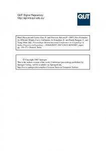
Experimental results – Shuffle-based multiplication 8000 This work (López-Dahab) This work (Shuffling) 7000


6000

5000

4000

3000

2000

1000

0 200

400

600

800

1000

1200

Field size

Note: Native multiplier on newer machines is twice faster than LD. Diego F. Aranha


Observations Squaring and square-root are: Efficiently formulated with M/S ratio up to 34 Faster when shuffling throughput is higher Heavily dependent on the choice of f (z) Shuffle-based multiplication: Has a bottleneck with constants stored in memory Requires faster table addressing scheme Is only 50%-90% slower than L´ opez-Dahab! Other operations: Restore the ratio to native multiplication (H ≈ M, I ≈ 25M).

Diego F. Aranha


Part III: Applications

Diego F. Aranha


Introduction

Elliptic Curve Cryptography (ECC): Underlying problem harder than integer factoring (RSA) Same security level with smaller parameters Efficiency in storage and execution time Pairing-Based Cryptography (PBC): Initially destructive Allows innovative protocols Flexibilizes curve-based cryptography

Diego F. Aranha


Introduction

Point multiplication is the most expensive operation in Elliptic Curve Cryptography. Pairing computation is the most expensive operation in Pairing-Based Cryptography. Parallelism is being increasingly introduced in modern architectures.

Diego F. Aranha


Objective Explore two types of parallelism in software to reduce computation latency: Vector instructions Multiprocessing Applications: desktop-class computers, real-time services, embedded devices. Contributions State-of-the-art timings for ECC and PBC Parallelization of Miller’s Algorithm with load balancing Experimental results

Diego F. Aranha


Elliptic curves

(a) Point addition R = P + Q;

(b) Point doubling R = 2P;

Figure : Elliptic curve arithmetic. [Picture: Hankerson et al. 2003]

Diego F. Aranha


Binary elliptic curves

A binary elliptic curve is the set of solutions (x, y ) ∈ F2m × F2m satisfying the equation y 2 + xy = x 3 + ax 2 + b, where a, b ∈ F2m with b 6= 0, and a point at infinity ∞. When a ∈ {0, 1} and b = 1, the curve is called a Koblitz curve.

Diego F. Aranha


Elliptic curves The set of points {(x, y ) ∈ E (F2m )} ∪ {∞} under the addition operation + (chord-and-tangent rule) forms an additive group. Given an elliptic point P and an integer k, the operation kP, called scalar multiplication, is defined by kP = P | + P +{z. . . + P.} k times

This is the fundamental operation employed by protocols based on elliptic curves. Important: Underlying problem: ECDLP: Recover k from hP, kPi.

Diego F. Aranha


Elliptic curve arithmetic

Algorithm 10 Double-and-add scalar multiplication P i Input: k = t−1 i=0 ki 2 , P ∈ E (F2m ) of order r . Output: kP. 1: Q ← ∞ 2: for i = t − 1 downto 0 do 3: Q ← 2Q 4: if ki = 1 then 5: Q ←Q +P 6: end if 7: end for 8: return Q

Diego F. Aranha


Elliptic curve arithmetic Algorithm 11 Left-to-right wNAF scalar multiplication Input: w , k ∈ Z, P ∈ E (F2m ) of order r . Output: kP. Pt−1 i 1: Obtain the representation NAFw (k) = i=0 ki 2 2: Compute Pi = iP for i ∈ {1, 3, . . . , 2w −1 − 1} 3: Q ← ∞ 4: for i = t − 1 downto 0 do 5: Q ← 2Q 6: if ki > 0 then 7: Q ← Q + Pki 8: else if ki < 0 then 9: Q ← Q − Pki 10: end if 11: end for 12: return Q Diego F. Aranha


Elliptic curve arithmetic Algorithm 12 Left-to-right multiple scalar multiplication Input: w , k ∈ Z, l ∈ Z, P ∈ E (F2m ) of order r . Output: kP + lQ. Pt−1 i P i 1: Obtain the representations NAFw (k) = t−1 i=0 li 2 i=0 ki 2 , NAFw (l) = 2: Compute Pi = iP, Qi = iQ for i ∈ {1, 3, . . . , 2w −1 − 1} 3: R ← ∞ 4: for i = t − 1 downto 0 do 5: R ← 2R 6: if ki > 0 then 7: R ← R + Pki 8: else if ki < 0 then 9: R ← R − Pki 10: end if 11: if li > 0 then 12: R ← R + Qli 13: else if li < 0 then 14: R ← R − Qli 15: end if 16: end for 17: return R

Important: With endomorphism ψ, compute kP = k1 P + k2 ψ(P). Diego F. Aranha



Koblitz curves have the Frobenius automorphism τ on E (F2m ) given by τ (x, y ) = (x 2 , y 2 ). If it is possible to recode k in another basis related to τ , point doublings can be replaced by applications of τ . Important: Many other approaches for scalar multiplication and other scenarios (fixed, multiple).

Diego F. Aranha


Elliptic curve arithmetic Algorithm 13 Left-to-right τ -and-add scalar multiplication Input: w , k ∈ Z, P ∈ E (F2m ) of order r . Output: kP. Pt−1 i 1: Obtain the representation TNAF (k) = i=0 ui τ 2: Q ← ∞ 3: for i = t − 1 downto 0 do 4: Q ← τQ 5: if ui = 1 then 6: Q ←Q +P 7: else if ui = −1 then 8: Q ←Q −P 9: end if 10: end for 11: return Q Diego F. Aranha


Elliptic curve arithmetic Algorithm 14 Left-to-right w τ NAF scalar multiplication Input: w , k ∈ Z, P ∈ E (F2m ) of order r . Output: kP. Pt i 1: Obtain the representation TNAFw (k) = i=0 ui τ 2: Compute Pu = αu P foru ∈ {1, 3, 5, . . . , 2w −1 − 1} where αi = i mod τ ω 3: Q ← ∞ 4: for i = t − 1 downto 0 do 5: Q ← τQ 6: if ui = αj , for some j then 7: Q ← Q + Pj 8: else if ui = −αj , for some j then 9: Q ← Q − Pj 10: end if 11: end for 12: return Q Diego F. Aranha


Elliptic curve arithmetic Algorithm 15 Constant-time point multiplication. P Input: k = t−1 i=0 ki ∈ Z, P = (x, y ) ∈ E (F2m ), b-coefficient. Output: kP ∈ E (F2m ). 1: x1 ← x, z1 ← 1, z2 ← x 2 , x2 ← z22 + b, 2: for i ← t − 2 to 0 do 3: r1 ← x1 z2 , r2 ← x2 z1 , r3 ← r1 + r2 , r4 ← r1 r2 4: if ki 6= 0 then 5: z1 ← r32 , r1 ← xz1 , x1 ← r1 + r4 , r1 ← z22 , r2 ← x22 6: z2 ← r1 r2 , x2 ← r12 , r1 ← r22 , r2 ← br1 , x2 ← x2 + r2 7: else 8: z2 ← r32 , r1 ← xz2 , x2 ← r1 + r4 , r1 ← z12 , r2 ← x12 9: z1 ← r1 r2 , x1 ← r12 , r2 ← r22 , r2 ← br1 , x1 ← x1 + r2 10: end if 11: end for 12: return Q = (x3 , y3 ) from (x1 /z1 , x2 /z2 ); Diego F. Aranha


Experimental results – Elliptic curve arithmetic

Table : Timings given in 103 cycles for side-channel resistant scalar multiplication.

Curve CURVE2251 - Core 2 CURVE2251 - CLMUL CURVE2251 - CLMUL + AVX BBE (Bernstein) - Core 2 eBACS (mpFq ) - Core 2 4-GLV-GLS TED (Longa) - Core i7

Diego F. Aranha

This work 594 282 225 Related work 314 855 137



Briefly recall that Koblitz curves have the Frobenius automorphism τ on E (F2m ) given by τ (x, y ) = (x 2 , y 2 ). Computing fixed powers 2k in constant time (independent of k) provides an endomorphism in the context of the GLV method. Let map ψ ≡ τ bm/2c , giving kP = k1 P + 2bm/2c k2 P = k1 P + k2 ψ(P). Interleaving saves b m2 c applications of the Frobenius. In general, exploiting the bm/sc-th power of τ is the analogue of an s-dimensional GLV decomposition and saves (s − 1)b ms c Frobenius. Note: Tables can be reused for fast Ito-Tsuji inversion.

Diego F. Aranha


Algorithm 16 Interleaved width-w τ NAF scalar multiplication. Input: k ∈ Z, P ∈ E (F2m ), integer s denoting the interleaving factor. Output: kP ∈ E (F2m ). P i 1: Compute width-w τ -NAF(k) = l−1 i=0 ui τ 2: Compute P0,u = αu P, for u ∈ {1, 3, 5, . . . , 2w −1 − 1} 3: for i ← 1 to (s − 1) do Compute Pi,u = τ bm/sc Pi−1,u 4: Q ← ∞ 5: for i ← l − 1 to sb ms c do 6: Q ← τQ 7: if ui 6= 0 then 8: Let u be such that αu = ui or α−u = −ui 9: if ui > 0 then Q ← Q + P0,u ; else Q ← Q − P0,u 10: end if 11: end for 12: for i ← (b ms c − 1) to 0 do 13: Q ← τQ 14: for j ← 0 to (s − 1) do 15: if ui+jbm/sc 6= 0 then 16: Let u be such that αu = ui+jbm/sc or α−u = −ui+jbm/sc 17: if ui > 0 then Q ← Q + Pj,u ; else Q ← Q − Pj,u 18: end if 19: end for 20: end for 21: return Q = (x, y )

Diego F. Aranha



Table : Timings given in 103 cycles for unprotected scalar multiplication.

Curve NISTK283 - CLMUL (w = 5, s = 2) NISTK283 - CLMUL + AVX (w = 5, s = 2) 4-GLV-GLS TED (Longa) - Sandy Bridge

Diego F. Aranha

This work 128 99 Related work 91


Bilinear pairings

Let G1 = hPi and G2 = hQi be additive groups and GT be a multiplicative group such that |G1 | = |G2 | = |GT | = prime n. An efficiently-computable map e : G1 × G2 → GT is an admissible bilinear map if the following properties are satisfied: 1

2

Bilinearity: given (V , W ) ∈ G1 × G2 and (a, b) ∈ Z∗q : e(aV , bW ) = e(V , W )ab = e(abV , W ) = e(V , abW ). Non-degeneracy: e(P, Q) 6= 1GT , where 1GT is the identity of the group GT .

Diego F. Aranha


Bilinear pairings

[Picture: Avanzi, Cesena 2009]

Diego F. Aranha


Bilinear pairings

If G1 = G2 , the pairing is symmetric. [Picture: Avanzi, Cesena 2009]

Diego F. Aranha


Example of protocol

Non-interactive ID-based key distribution protocol [SOK 2000]: A trusted authority generates master key s; An user i receives IDi , hPi = h(IDi ), Si = sPi i; Users A and B can derive the same key e(SA , PB ) = e(SB , PA ) = e(PA , PB )s . Important: Underlying problem: BCDHP: Compute e(P, Q)abc from hP, aP, bP, cP, Q, aQ, bQ, cQi.

Diego F. Aranha


Pairing computation

Let P, Q be r -torsion points. The pairing e(P, Q) is defined by the evaluation of fr ,P at a divisor related to Q. [Miller 1986] constructed fr ,P in stages combining Miller functions evaluated at divisors. [Barreto et al. 2002] showed how to evaluate fr ,P at Q using the final exponentiation employed by the Tate pairing.

Diego F. Aranha


Pairing computation

Let gU,V be the line equation through points U, V ∈ E (Fqk ) and gU the shorthand for gU,−U . For any integers a and b, we have: 1

fa+b,P (D) = fa,P (D) · fb,P (D) ·

2

f2a,P (D) = fa,P (D)2 ·

3

fa+1,P (D) = fa,P (D)

gaP,bP (D) ; g(a+b)P (D)

gaP,aP (D) g2aP (D) ; g (D) · g (a)P,P (D) . (a+1)P

Diego F. Aranha


Pairing computation Algorithm 17 Miller’s Algorithm [Miller 1986, Barreto et al. 2002]. Plog r Entrada: r = i=02 ri 2i , P, Q. Sa´ıda: er (P, Q). 1: T ← P 2: f ← 1 3: r ← r − 1 4: for i = blog2 (r )c − 1 downto 0 do 5: f ← f 2 · lT ,T (Q) 6: T ← 2T 7: if ri = 1 then 8: f ← f · lT ,P (Q) 9: T ←T +P 10: end if 11: end for k 12: return f (q −1/r ) Diego F. Aranha


Related work

Scalable approaches: [Mitsunari 2009] and [Beuchat et al. 2009] precompute pairs (Ti , part of lTi ,Ti (Q)) in the symmetric case and divide loop iterations among processors. Problem: High storage costs (large precomputation).

Diego F. Aranha


New approach Property of Miller functions fa·b,P (D) = f b,P (D)a · f a,bP (D) We can write r = 2w r1 + r0 and compute fr ,P (D): fr ,P (D) = f2w r1 +r0 ,P (D) w

= f r1 ,P (D)2 · f 2w ,r1 P (D) · f r0 ,P (D) ·

g(2w r1 )P,r0 P (D) . grP (D)

If r has low Hamming weight, w can be chosen so that r0 is small. For many processors, we can: Apply the formula recursively: Write r as r = 2wi ri + · · · + 2w2 r2 + 2w1 r1 + r0 . If P is fixed (private key), ri P can also be precomputed. Diego F. Aranha


Load balancing

Problem: We must determine an optimal partition wi . Let c1 (1) the cost of a serial loop and cπ (i) the cost of a parallel loop for processor 1 ≤ i ≤ π. We can count the operations executed by each processor and solve the system cπ (1) = cπ (i) to obtain wi . The speedup is: s(π) =

c1 (1)+exp cπ (1)+par +exp ,

where par is the cost of parallelization and exp is the cost of the final exponentiation.

Diego F. Aranha


Symmetric case – Elliptic curves

A pairing-friendly supersingular binary elliptic curve is the set of solutions (x, y ) ∈ F2m × F2m satisfying the equation y 2 + y = x 3 + x + b, where b ∈ {0, 1}, and a point at infinity ∞. m+1

The order of this curve is N = 2m + 1 ± 2 2 and the embedding degree is k = 4 (the least integer such that N divides 2km − 1).

Diego F. Aranha


Symmetric case – Pairing definition

Choosing T = 2m − N and a prime r dividing N, [Barreto et al. 2004] defined the reduced ηT pairing: ηT

:

E (F2m )[r ] × E (F2m )[r ] → F∗24m

ηT (P, Q) = fT 0 ,P 0 (ψ(Q))

24m −1 N

,

where T 0 = ±T and P 0 = ±P. The function f is a Miller function and ψ is the distortion map ψ(x, y ) = (x 2 + s, y + sx + t).

Diego F. Aranha


Symmetric case – Pairing algorithm Algorithm 18 ηT pairing [Barreto et al. 2004], [Beuchat et al. 2008]. Input: P = (xP , yP ), Q = (xQ , yQ ) ∈ E (F2m )[r ]. Output: ηT (P, Q) ∈ F∗24m .

1: yP ← yP + 1 − δ 2: u ← xP + α, v ← xQ + α 3: g0 ← u · v + yP + yQ + β 4: g1 ← u + xQ , g2 ← v + xP2 5: G ← g0 + g1 s + t 6: L ← (g0 + g2 ) + (g1 + 1)s + t 7: F ← L · G do 8: for i ← 1 to m−1 2 √ √ 9: xP ← xP , yP ← yP , xQ ← xQ2 , yQ ← yQ2 10: u ← xP + α, v ← xQ + α 11: g0 ← u · v + yP + yQ + β 12: g1 ← u + xQ 13: G ← g0 + g1 s + t 14: F ←F ·G 15: end for m+1 2m m 16: return F (2 −1)(2 +1±2 2 )

Diego F. Aranha


Symmetric case – Parallel pairing Algorithm 19 Proposed parallel ηT pairing. Input: P = (xP , yP ), Q = (xQ , yQ ) ∈ E (F2m )[r ]. Output: ηT (P, Q) ∈ F∗24m .

1: parallel section(processor i) 2: if i = 1 then Initialize F1 as in lines 1-7 of the previous algorithm; 3: else Fi ← 1 1 1 w w 4: xP i ← (xP ) 2wi , yP i ← (yP ) 2wi , xQ i ← (xQ )2 i , yQ i ← (yQ )2 i 5: for j ← wi to wi+1 − 1 do √ √ 6: xP i ← xP i , yP i ← yP i , xQ i ← xQ 2i , yQ i ← yQ 2i 7: ui ← xP i + α, vi ← xQ i + α 8: g0i ← ui · vi + yP i + yQ i + β 9: g1i ← ui + xQ i 10: Gi ← g0i + g1i s + t 11: Fi ← Fi · Gi 12: end for Q 13: F ← πi=1 Fi 14: end parallel 15: return F M

Note: If memory is available, use partitions with the same size. Diego F. Aranha


Experimental results – Speedup (45nm) 14 12

Beuchat et al. 2009 Aranha et al. 2010

Speedup

10 8 6 4 2 0

10

20

30

40

50

Number of processors

Diego F. Aranha


60

Experimental results – Latency (45nm)

Latency (millions of cycles)

30 25

Beuchat et al. 2009 Aranha et al. 2010 23.03

20

17.40

15

13.14 9.34

10

9.08

8.93 5.08

5 0

3.02

1

2

4 Number of threads

Diego F. Aranha

8


Conclusions New formulation and implementation of binary field arithmetic: Follows trend of faster shuffle instructions Improve results from related work by 8%-84% Induces a new implementation strategy for multiplication Still requires architectural features to be optimal May be cheaper to support than a full native multiplier Timings for non-batched arithmetic on binary elliptic curves: Provide new speed record for side-channel resistant scalar multiplication on binary curves Improve results for kP on eBACS by at least 27%-30%

Diego F. Aranha


Conclusions New state-of-the-art for parallel implementation of pairings: No significant storage costs, smaller precomputation; In comparison with our serial implementation, speedups of 46%, 70% and 83% with 2, 4 and 8 cores; In comparison with previous state-of-the-art, improvements in latency of 24%, 29%, 44% and 66% with 1, 2, 4 and 8 cores. Parallelization scales: In the covered case, point doublings and extension field squarings are efficient; Our finite field implementation make these exceptionally fast.

Diego F. Aranha


Detailed results Platform 1 – Intel Core 2 65nm Hankerson et al. – latency Beuchat et al. – latency Beuchat et al. – speedup This work – latency This work – speedup Improvement Platform 2 – Intel Core 2 45nm Beuchat et al. – latency Beuchat et al. – speedup This work – latency This work – speedup Improvement Platform 3: Intel Core i7 32nm This work – latency This work – speedup Improvement

1 39 26.86 1 18.76 1 30.2% 1 23.03 1 17.40 1 24.4% 1 6.46 1.00 62.3%

Number of threads 2 4 – – 16.13 10.13 1.67 2.65 10.08 5.72 1.86 3.28 32.9% 39.9% 2 4 13.14 9.08 1.77 2.54 9.34 5.08 1.86 3.42 28.9% 44.0% 2 4 3.37 1.79 1.92 3.60 63.9% 64.8%

Table : Timings are reported in millions of cycles. Diego F. Aranha


8* – – – 3.55 5.28 – 8 8.93 2.58 3.02 5.76 66.2% 8* 1.03 6.24 65.9%

Sources [1] D. F. Aranha, J. L´ opez, D. Hankerson, “High-speed parallel software implementation of the ηT pairing”, In CT-RSA 2010, Springer LNCS 5985, pp. 89–105, San Francisco, USA, 2010. [2] D. F. Aranha, J. L´ opez, D. Hankerson, “Efficient Software Implementation of Binary Field Arithmetic Using Vector Instruction Sets”, In LATINCRYPT 2010. Springer LNCS 6212, pp. 144–161, Puebla, Mexico, 2010. [3] J. Taverne, A. Faz-Hern´ andez, D. F. Aranha, F. Rodr´ıguez-Henr´ıquez, D. Hankerson, J. L´ opez, “Software implementation of binary elliptic curves: impact of the carry-less multiplier on scalar multiplication”, In CHES 2011, Springer LNCS 6917, pp. 108–123, Nara, Japan, 2011. [4] J. Taverne, A. Faz-Hern´ andez, D. F. Aranha, F. Rodr´ıguez-Henr´ıquez, D. Hankerson, J. L´ opez, “Speeding scalar multiplication over binary elliptic curves using the new carry-less multiplication instruction”, Journal of Cryptographic Engineering, Vol. 1, Number 3, pp. 187–199, 2011. [5] D. F. Aranha, E. Knapp, A. Menezes, F. Rodr´ıguez-Henr´ıquez, “Parallelizing the Weil and Tate pairings”, In IMACC 2011, Springer LNCS 7089, pp. 275–295, Oxfork, UK, 2011. [6] D. F. Aranha, A. Faz-Hern´ andez, J. L´ opez, F. Rodr´ıguez-Henr´ıquez, “Faster Implementation of Scalar Multiplication on Koblitz Curves”, In LATINCRYPT 2012, Springer LNCS 7533, pp. 177–193, Santiago, Chile, 2012. Diego F. Aranha
