Jan 1, 2000 - As a member of the Cay- ley graphs, the star graph possesses several attractive features such as its diameter-to-node-degree ratio, scal- ability ...
IEICE TRANS. FUNDAMENTALS, VOL.E83–A, NO.1 JANUARY 2000
139
PAPER
Efficient Broadcasting in an Arrangement Graph Using Multiple Spanning Trees∗ Yuh-Shyan CHEN† , Tong-Ying JUANG†† , and En-Huai TSENG† , Nonmembers
SUMMARY The arrangement graph An,k is not only a generalization of star graph (n − k = 1), but also more flexible. Designing efficient broadcasting algorithm on a regular interconnection network is a fundamental issue for the parallel processing techniques. Two contributions are proposed in this paper. Initially, we elucidate a first result to construct n − k edge-disjoint spanning trees in an An,k . Second, we present efficient (one/all)to-all broadcasting algorithms by using constructed n − k spanning trees, where height of each spanning tree is 2k − 1. The arrangement graph is assumed to use one-port and all-port communication models and packet-switching (or store-and-forward) technique. Using n − k spanning trees allows us to present efficient broadcasting algorithm in the arrangement graphs and outperforms previous results. This is justified by our performance analysis. key words: arrangement graph, broadcast, interconnection network, parallel processing, routing
1.
Introduction
Designing large multi-processor systems frequently involves organizing into various configurations. One of the widely studied interconnection network topologies is the star graph [9], [11], [12]. As a member of the Cayley graphs, the star graph possesses several attractive features such as its diameter-to-node-degree ratio, scalability, partitionability, symmetry, and high degree of fault tolerance [1], [3]. However, the star graph is limited with respect to its number of nodes: n! for an n-dimensional star graph. A new interconnection topology, arrangement graph, has recently been proposed [4]. As a family of undirected graphs that contains the star graph family, the arrangement graph has desired properties, such as symmetric vertex and symmetric edge, strongly resilience and maximally fault-tolerance. Arrangement graph is more flexible than the star graph in terms of choosing major design parameters, i.e. member of vertices, degree and diameter, while preserving most of the excellent properties of the star graph. Manuscript received April 19, 1999. Manuscript revised August 16, 1999. † The authors are with the Department of Computer Science and Information Engineering, Chung-Hua University, Hsin-Chu, 30067, Taiwan, Republic of China. †† The author is with the Department of Statistics, National Chung Hsing University, Taipei, Taiwan, Republic of China. ∗ This paper was presented at ICPADS ’98 conference, and this work was supported by the National Science Council, R.O.C., under Contract NSC88-2213-E-216-011.
The arrangement graph has received considerable attention in [2], [4]–[8], [10]. Firstly, Day and Tripathi [5] designed a shortest-path routing algorithm for the arrangement graphs. According to their results, the arrangement graph can be embedded cycles whose length ranging from three to the size of the graph [6]. Moreover, the arrangement graph can be decomposed into vertex disjoint cycles in many different ways [6]. Furthermore, multi-dimensional grads, hypercube and one spanning tree can be embedded in arrangement graph [7]. The spanning tree can support broadcasting communication in the arrangement graph. Tsai and Horng proposed an efficient scheme to embed hypercube on arrangement graphs [10]. Heieh and Chen [8] further demonstrated that the arrangement graph remains a ring even if it is faulty. Bat et al. [2] recently proposed a distributed fault-tolerant algorithm for oneto-all broadcasting only in the one-port communication model on the arrangement graph. In light of above discussion, this work elucidates the broadcast problem on arrangement graphs in oneport and all-port communication model. In this work, the network adopts the packet-switching or store-andforward technique. By following the formulation of many works (e.g. [13]), assume the existence of two kinds of cost: start-up time and transmission time. In particular, a packet of b bytes is sent along a link takes Ts +bTc time, where Ts denotes the time to initialize (or start-up) the communication link and Tc represents the latency to transmit a byte. An attempt to minimize either the start-up time cost and the transmission cost is the underlying motivation of this work. Typically, the start-up time is significant in current machines, while the transmission time should not be neglect when the packet is long. Note that Bat et al. [2] proposed broadcast algorithm only optimize the start-up time, but not consider the transmission time. In contrast to earlier solution in arrangement graph [2], [7], this work aims to minimize start-up time and transmission costs simultaneously. The major approach used herein is to construct multiple spanning trees. For the broadcasting algorithm, we propose a new scheme to construct multiple spanning trees in an arrangement graph An,k that has a desired property that n − k copies of such trees can be embedded simultaneously in the network without edgecongestion. By concurrently transmitting data along
IEICE TRANS. FUNDAMENTALS, VOL.E83–A, NO.1 JANUARY 2000
140
these trees in a pipelined manner, our results are an improvement over the schemes of deriving one spanning tree in [7] by order O(n − k) in the transmission time. In this investigation, we assume that a node consists of a processor with bidirectional communication links to each of its adjacent nodes. Therefore, the term edgedisjoint spanning trees can be interchangeably adopted to reflect that no two edges of our spanning trees share a same direct communication link. To our knowledge, this work reports for the first time on feasibility of embedding multiple O(n−k) spanning trees in an An,k while, at the same time, keeping the edge-congestion free. Similar results for the star graph can be found in [13]. A broadcast algorithm is proposed herein by the subgraph-partitioning scheme. Under the all-port model, the proposed one-toall broadcast algorithm can be executed in An,k in time � � mTc 2 ( (2k − 1)Ts + n−k ) , where m denotes the size of the broadcast message. Under the one-port model, the one-to-all broadcast algorithm can be implemented in An,k in time O(k(n − k)(2k − 1)Ts + kmTc ). Under the all-port model, the all-to-all broadcast algorithm can be mn! Tc ). implemented in An,k in time O(2k×Ts + (n−k)(n−k)! Under the one-port model, the all-to-all broadcast algorithm can be performed in An,k in time O(2k 2 (n − kmn! k)Ts + (n−k)! Tc ). The rest of this paper is organized as follows. Section 2 introduces preliminaries. Section 3 presents how to construct multiple spanning trees. Section 4 compares our broadcasting results with those of other related works. Conclusions are finally drawn in Sect. 5. 2.
Preliminaries
The arrangement graph is denoted by An,k , where specified by integers n and k and � � 1 ≤ k ≤ n − 1. Denote �n� = {1, 2, . . . , n}. Let P nk be the set of permutations of k symbols taken from �n�. These k symbols are denoted as X = x1 x2 · · · xk . Refer xi as the i’th element of X. The (n, k)-arrangement graph, denoted as An,k , defined in [5] is an undirected graph (V, E) as follows. V = {X = x1 x2 · · · xk |xi in �n� and xi = xj for � � i = j} = P nk }, E = {(x, y)|x and y in V and for some i in �k� xi = yj and xj = yj for j = i}. Figure 1 depicts an example of A4,2 and A5,3 . The edge of An,k connecting neighboring nodes which differ in exactly one of their k positions. The vertices of An,k are the arrangements of k elements of �n�. For example, in A4,2 , the node p = 41 is connected to the nodes = 42, 43, 21 and 31. An edge of An,k connecting two arrangements p and q which differ only in position i, is called as an i-edge. For all values
n! nodes of n and k, An,k is a regular graph on (n−k)! that 3 is regular of degree k(n − k), and a diameter 2 k [5]. For an arrangement X = x1 x2 . . . xk , we define EXT (X) = �n� − {x1 , x2 , . . . , xk } to be the n − k elements of �n� not appearing in the arrangement X. Let INT (X) = {x1 , x2 , . . . , xk } = �n� − EXT (X) to be the k elements of appearing in the arrangement X. For example, we consider the node p = 412 in the arrangement graph A5,3 , so EXT (p) = {3, 5} and INT (p) = {1, 2, 4}. In an An,k , each node p performs an adjacent function ADJ x,y (p) to arrive at adjacent node q, where x is the position of label of node and y is the changed label in EXT (p). Given X = x1 · · · xx · · · xk ∈ IN T (X), the adjacent function ADJx,y (X) is the adjacent nodes of X obtained by changing xx in X to be y, where 1 ≤ x ≤ k and y ∈ EXT (X). Consider an A5,3 , adjacent nodes for node p = 412 are 413, 415, 432, 452, 312 and 512, where EXT (p) = {3, 5}, INT (p) = {1, 2, 4}, ADJ 1,3 (p) = 312, ADJ 1,5 (p) = 512, ADJ 2,3 (p) = 432, ADJ 2,5 (p) = 452, ADJ 3,3 (p) = 413, and ADJ 3,5 (p) = 415. The An,k is with recursive structure [5]. That is, an An,k can be partitioned into n copies of An−1,k−1 each embedded An−1,k−1 is conveniently denoted by n,k , where α ∈ {1, 2, · · · , n}, (where ∗ represents a “don’t care” symbol). For example, 4,3 represents an embedded A3,2 of A4,3 , contains six nodes: 123, 143, 213, 243, 413, and 423. From other point of view, there are n copies of n,k which are obtained by performing a splitting operation on n,k , where α ∈ {1, 2, . . . , n}. This operation is called as k-partition. Generally, An,k can be partin! tioned into (n−p)! node-disjoint copies of An−p,k−p in n! different ways and that in total An.k contains � n! �p!(n−p)! k p (n−p)! copies of An−p,k−p , for 1 ≤ p ≤ k − 1. In this paper, we adopt the packet-switching (or store-and-forward) model and, thus, the latency to transmit a packet of b byte along a link is Ts + bTc , where Ts denotes the time to initialize the communication link and Tc represents the time to transmit a byte. Each (undirected) edge is regarded as bidirectional communication links. Two communication models are also considered. In the one-port model, a node can send and receive at most one packet at a time. While in the all-port model, a node can simultaneously send and receive a packet along all k(n − k) ports.
Lemma 1: A lower bound for one-to-all � broadcasting m Tc in a store-and-forward An,k is max 32 k Ts , k(n−k) �
under the all-port model, and max 32 k Ts , n!
log (n−k)! �Ts , mTc under the one-port model, where m is the size of the broadcast message. Lemma 2: A lower bound for all-to-all broadcast-
CHEN et al: BROADCASTING IN ARRANGEMENT GRAPH
141
(a)
(b) Fig. 1
An example of arrangement graphs (a) A4,2 and (b) A5,3 .
�
ing in a store-and-forward An,k is max 32 k Ts , n! m under the all-port model, and · T c (n−k)! � k(n−k)
n! n! max 32 k Ts , log (n−k)! �Ts , (n−k)! · mTc under the one-port model, where m denotes the size of the broadcast message. 3.
Congestion-Free Embedding of Multiple Spanning Trees
This section presents a scheme to embed n − k edgedisjoint spanning trees in an An,k . Our construction scheme adopts a bottom-up manner. An An,k can n! copies of An−k+2,2 . Each be partitioned into (n−k+2)!
An−k+2,2 initially construct n − k base spanning trees. For each An−k+3,3 , there are n−k+3 copies of An−k+2,2 and each one containing n − k base spanning trees. We propose a concatenation operation to construct larger n − k spanning trees in an An−k+3,3 . Recursively performing the concatenation operations allow us to finally construct n − k spanning trees in an An,k . Our n − k spanning trees are constructed by two phases: • Phase 1: Generate n − k base spanning trees in each An−k+2,2 . • Phase 2: Perform a recursive concatenation operation to embed n − k edge-disjoint spanning trees. These phases are described as follows.
IEICE TRANS. FUNDAMENTALS, VOL.E83–A, NO.1 JANUARY 2000
142
3.1 Phase 1: Generate n − k Base Spanning Trees in an An−k+2,2 n! After a splitting-operation on An,k , (n−k+2)! copies of An−k+2,2 ’s are obtained. According to different values of n and k, n − k base spanning trees in each An−k+2,2 can be generated as follows.
• Step 1: Locate n − k roots nodes. • Step 2: Generate n − k base spanning trees in each An−k+2,2 . 3.1.1
Step 1: Locating n − k Roots in an An−k+2,2
We now describe how to locate n − k root nodes in an An−k+2,2 . Initially, we let each An−k+2,2 be partitioned into n − k + 2 copies of An−k+1,1 , where each An−k+1,1 is a (n − k + 1)-node complete graph. Denote these n − k root nodes as R1 , R2 , . . ., and Rn−k as follows. Let R1 = (y1 x2 x3 · · · xk ) be any node in an An−k+1,1 . Other root nodes R2 = (y2 x2 x3 · · · xk ), R3 = (y3 x2 x3 · · · xk ), . . ., and Rn−k+1 = (yn−k+1 x2 x3 · · · xk ) by exchanging the first bit of R1 with α, where α ∈ EXT (R1 ) = {y2 , . . . , yn−k+1 }. This task can be achieved as follows.
(a) Fig. 2
(b)
Two base edge-disjoint spanning trees in an A4,2 .
Ri = ADJ 1,α (R1 ), where 2 ≤ i ≤ n − k + 1 and α ∈ EXT (R1 ). Each pair of R1 , R2 , . . ., and Rn−k+1 are adjacent since R1 , R2 , . . ., and Rn−k+1 belong to an An−k+1,1 (a complete graph ∗x2 x3 · · · xk ). Note that node Rn−k+1 is used to as a template node to ensure congestion-free in our embedding. Intuitively, every Ri is only different in the first bit. Root nodes Ri , 1 ≤ i ≤ n − k, are selected from ∗x2 x3 · · · xk . Clearly, ∗x2 x3 · · · xk is an An−k+1,1 or (n−k+1)-node complete graph. Root nodes R1 , R2 , . . ., Rn−k satisfy the root-location property. This rootlocation property is very useful during constructing n − k spanning trees. Root-Location Property: There are n − k root nodes Ri , 1 ≤ i ≤ n − k, in same subarrangement graph. Root nodes Ri , i = 1..n − k, belong to an An−k+1,1 . Root nodes Ri , i = 1..n − k, are used to expand n − k base spanning trees in an An−k+2,2 . Figure 2 illustrates an example that four root nodes are 21 and 31. Template node is 41. 3.1.2
Step 2: Generate n−k Base Edge-Disjoint Spanning Trees in an An−k+2,2
We now describe how to construct n − k base spanning trees from root Ri , 1 ≤ i ≤ n − k, for every An−k+2,2 . The height of base spanning tree is 3. The fact that
(a)
(b)
(c)
(d)
Fig. 3 Four disjoint spanning trees whose tree height = 1 in a 4-node complete graph.
each An−k+1,1 is a complete graph accounts for why n − k base spanning trees can be constructed if we can connect each root nodes to distinct node of all other An−k+1,1 ’s. This is because that we have the following result and Fig. 3 gives an example. Lemma 3: For a κ-node complete graph G, there exist κ disjoint spanning trees with height one. Notably, each node in G is the root node of each spanning tree. Now we explain how to construct n − k base spanning trees in each An−k+2,2 . As stated in Sect. 2, a ndimensional arrangement graph contains n subarrangements that we use to derive the desired spanning trees. Given n − k root nodes Ri , 1 ≤ i ≤ n − k, let R be one of these; we must connect R to other n − 1 subarrangements. For node R, we use a single edge to connect the R to n − k of subarrangements. We use an intermediate node in same subarrangement as the bridge node to
CHEN et al: BROADCASTING IN ARRANGEMENT GRAPH
143
connect R to the remaining k − 1 subarrangements by two edges. If k = 2, then there is only one subarrangement connecting by two edges. Rules A1 and A2 formalize the construction. A1: (Single edge) Let node R˙ denote connected node in every n − k subarrangements. R˙ = ADJ 2,α (R), where α ∈ EXT (R). ¨ denote connected node A2: (Two edges) Let node R in one of remaining k − 1 subarrangements which connected by two edges (Note that in this case, k = 2). Recall in phase 1, node Rn−k+1 is the intermediate nodes for node R.
(a)
¨ = ADJ 2,β (Rn−k+1 ), where β is the first bit R value in R. Figure 2 (a) shows that root node 21 uses distinct single edge to connecting nodes 23 and 24, and connecting node 42 by ADJ 2,2 (41), where node 41 is template node. Figure 2 (b) displays that root node 31 directly connects to 32 and 34 but connects 43 by ADJ 2,3 (41). Now we verifies the correctness of n − k base spanning trees in an An−k+2,2 . Some notations are defined firstly. Given root nodes Ri , 1 ≤ i ≤ n − k, are constructed by phase 1 of Sect. 3. An An−k+2,2 can be partitioned into n − k + 2 copies of An−k+1,1 or A�n−k+1,1 along dimension two or one. First, let an An−k+2,2 be partitioned into n − k + 2 copies of An−k+1,1 along second dimension. Root nodes Ri , 1 ≤ i ≤ n − k, located in one of An−k+1,1 . Let IE(Ri ), 1 ≤ i ≤ n−k, denote a set of all possible internal edges within every An−k+1,1 . Let EE(Ri ) denote a set of all possible external edges outgoing every An−k+1,1 . For example as illustrated in Fig. 4 (a), all bold edges are IE(Ri ) and all dash edges are EE(Ri ). Similarly, the same An−k+2,2 can be partitioned into n − k + 2 copies of A�n−k+1,1 along first dimension as shown in Fig. 4 (b). Some important properties are used later as stated herein. For 1 ≤ i ≤ n − k, we have following properties. P1: Edges in IE(Ri ) and edges in EE(Ri ) are equal to all edges in the An−k+2,2 . P2: Edges in IE(Ri ) and edges in EE(Ri ) are distinct. Lemma 4: There exist n − k edge-disjoint spanning trees STn−k+2,2 (Ri ) in an An−k+2,2 , for 1 ≤ i ≤ n − k. Proof. Given root nodes Ri , 1 ≤ i ≤ n − k, are located in one of partitioned An−k+1,1 . Every root node needs to connect to other An−k+1,1 . Therefore, n−k spanning trees STn−k+2,2 (Ri ), for 1 ≤ i ≤ n − k, are mutually disjoint due to the fact that every root node satisfy the following conditions: 1: All edges of R1 , R2 , . . ., and Rn−k connecting to the same An−k+1,1 are disjoint. 2: All nodes in the same An−k+1,1 connecting to R1 , R2 , . . ., and Rn−k differ from each other.
(b) Fig. 4 Edge distribution in an A4,2 ; (a) all internal edges within each A3,1 in A4,2 , (b) all internal edges within each A�3,1 in A4,2 .
The reason is stated as follows. Recalled again, since k = 2, for all Ri , we use n − 2 distinct single edges connecting to n − 2 copies of An−k+1,1 and use two edge to connect with remaining one An−k+1,1 . Intuitively, all edges connecting from R1 , R2 , . . ., and Rn−k to template node Rn−k+1 are distinct since all of these nodes located in a (n − k + 1)-node complete graph (or An−k+1,1 ). Recall previous notation, edges in all possible An−k+1,1 are denoted as IE(Ri ) and all edges in all possible A�n−k+1,1 are denoted as EE(Ri ). For condition 1, all edges of R1 , R2 , . . ., and Rn−k connecting to the same An−k+1,1 are disjoint because every edge belongs to different A�n−k+1,1 . Remember, these edges are belong to EE(Ri ). For condition 2, all nodes in the same An−k+1,1 connecting to R1 , R2 , . . ., and Rn−k differ from each other due to the fact that each of these ✷ nodes belongs to distinct A�n−k+1,1 . Theorem 5: There exist n − k base edge-disjoint spanning trees STn−k+2,2 (Ri ) in an An−k+2,2 , where 1 ≤ i ≤ n − k. Each spanning tree’s height is 3.
IEICE TRANS. FUNDAMENTALS, VOL.E83–A, NO.1 JANUARY 2000
144
(a)
(b) Fig. 5 Example of two spanning trees in an A5,3 ; (a) from root node 215, (b) from root node 315.
3.2 Phase 2: Construction of n − k Edge-Disjoint Spanning Trees in an An,k The above section constructed n−k base spanning trees in An−k+2,2 , and each base spanning tree’s height is 3. In this section, we describe how to construct n − k spanning trees STn,k (Ri ), for 1 ≤ i ≤ n − k in an An,k , where the height of each spanning tree is 2k − 1. For induction, we construct n − k spanning trees in an An,k by using n(n − k) spanning tress in n copies of An−1,k−1 . Our major task is to connect n(n − k) spanning subtrees into n − k spanning trees STn,k (Ri ), 1 ≤ i ≤ n − k. Consider an An,k which is partitioned into n copies of An−1,k−1 . Assume that n − k spanning trees STn−1,k−1 (Ri ), i = 1..n − k, can be constructed in each An−1,k−1 if their root nodes satisfied the root-location property. A randomly selected An−1,k−1 servers as beginning spanning tree. From this An−1,k−1 , there exist n − k spanning trees STn−1,k−1 (Ri ), 1 ≤ i ≤ n − k,
where Ri are root nodes. Let root node Ri connect to root node Ri� , where Ri� located in one of other An−1,k−1 . If Ri� satisfy the root-location property, then we can correctly construct n − k spanning trees STn,k (Ri ), 1 ≤ i ≤ n − k, in an An,k . As similar work mentioned in phase 1. A ndimensional arrangement graph contains n subarrangements that we use to derive the desired spanning trees. Given n − k root nodes Ri , 1 ≤ i ≤ n − k, let R are one of these; we must connect R to other n − 1 subarrangements. For each R, we use a single edge to connect the R to n−k of subarrangements. We also use an intermediate node in same subarrangement as the bridge node to connect R to the remaining k − 1 subarrangements by two edges. Rules A1’ and A2’ formalize our recursively spanning tree construction. A1’: (Single edge, the part is same as A1.) Let node R˙ denote connected node in every n − k subarrangements. R˙ = ADJ 2,α (R), where α ∈ EXT (R).
CHEN et al: BROADCASTING IN ARRANGEMENT GRAPH
145 �
which can directly connected to n,k by two edges. This is owing to that if root nodes Ri are n,k , root nodes Ri� are obtained by n,k ↔
¨ A2’: (Two edges, this part is same as A2.) Let node R denote connected node in one of remaining k − 1 subarrangements which connected by two edges. Nodes Rn−k+1 is the intermediate node for node R.
¨ = ADJ 2,β (Rn−k+1 ), where β is the first bit R value in R.
n,k
↔
�
n,k , where 1 ≤ i ≤ j
��
�
k−2
n − k, 1 ≤ j ≤ k − 2. Intuitively, Ri� are n,k , which differ in one bit,
j
��
k−2
�
so satisfy the root-location property. Figure 6 (c) provides an example, root node 215 ↔ 245 ↔ 241 and root node 315 ↔ 345 ↔ 341, where 241 and 341 ∈ 5,3 . ✷
Lemma 6: There are n − k root nodes Ri� , 1 ≤ i ≤ n − k, in same subarrangement graph are satisfied the root-location property. Proof. There are n subarrangements n,k , where β ∈ . One of the subarrangements n,k is selected as base spanning trees. In addition, let root nodes R1 , R2 , . . ., and Rn−k belong to a An−k+1,1 denoted as n,k , where α ∈ − {∗k−2 β � } − {t} and let n,k be a template node. Our results demonstrate that root nodes � in each An−1,k−1 also belong to R1� , R2� , . . ., and Rn−k a distinct An−k+1,1 . Three cases are discussed as follows.
k−2
∗ · · · ∗ ��� t ∗···∗
Figure 5 illustrates that two spanning trees in an A5,3 , where root nodes are 215 and 315. Assume that Ri� , 1 ≤ i ≤ n − k, are new connecting root nodes in each of other (n − 1)-subarrangement. Ensuring that root nodes Ri� satisfied the root-location property would allow us to establish our spanning trees STn,k (Ri ), for i = 1..n − k. In lemma 5, we show the correctness that root nodes Ri� satisfied root-location property, for i = 1..n − k.
j
��
Lemma 7: The height of n−k edge-disjoint spanning trees STn,k (Ri ) in an An,k is 2k − 1. Proof. There are k steps to construct STn,k (Ri ), 1 ≤ i ≤ n − k. Each step needs at most two edges except that the final step in An−k+1,1 needs one single edge since An−k+1,1 is a complete graph. The height is 2(k − 1) + 1 = 2k − 1. ✷ Theorem 8: There exist n− k edge-disjoint spanning trees STn,k (Ri ) with height 2k − 1 in an An,k , where i = 1..n − k. Proof. See proof in lemmas 6 and 7. ✷ The fact that there existing n − k edgedisjoint spanning trees STn,k (R1 ), STn,k (R2 ), . . ., and STn,k (Rn−k ) in an An,k with height 2k − 1. The fact that each pair of root nodes R1 , R2 , . . ., and Rn−k are adjacent allows us to logical construct a broadcast tree with height 2k. Note that we use the template node Rn−k+1 as the new root node of the logical broadcast tree. Consequently, a broadcasting algorithm using n−k edge-disjoint spanning trees can be obtained. The detailed algorithm is given in the next section. 4.
Broadcast Analysis
Algorithm
and
Performance
One-to-all broadcast refers to the problem of sending a message from a source node to all other nodes in the network. All-to-all broadcast refers to the problem of sending a message from all source nodes to all other nodes in the network. Two communication models are considered as follows.
IEICE TRANS. FUNDAMENTALS, VOL.E83–A, NO.1 JANUARY 2000
146
(a)
(b)
(c) Fig. 6
Example of proof in Lemma 6.
4.1 Under All-Port Model In the proposed algorithm, time is slotted by a fixed length and all nodes in the network are assumed to broadcast synchronously. In each time slot, each node
m , where m detransmits a packet of a fixed size p(n−k) notes the size of message M and p represents an integer be determined later. Therefore, each time slot is of m Tc . length Ts + p(n−k) Algorithm 1: /* One-to-all-broadcast, all-port */
CHEN et al: BROADCASTING IN ARRANGEMENT GRAPH
147
1) Divide the message M evenly into p(n − k) parts, each called a “message segment ” and of size m p(n−k) . 2) In each time slot, node r issues n − k message segments to the network, each along one of the trees STn,k (Ri ), i = 1..n − k. A message segment is then propagated along the tree it is issued. Each time slot helps propagate all message segments it received in the previous time slot to the subsequent nodes in the corresponding trees. Next, we analyze the communication latency of the algorithm. Notably, our analysis neglects the computational time (such as making routing decision or packing/unpacking packets). Let h be the maximal height of STn,k (Ri ), i = 1..n − k. The broadcast algorithm run in time � � m Tc T = h Ts + p(n − k) � � m Tc , + (p − 1) Ts + p(n − k) where h = 2k (1) The former term is the time for the first packet to arrive at the bottom of the tallest tree and the latter term is due to the pipeline effect. To minimize Eq. (1), let the derivative of T with respect to p equal 0, m ∂T = Ts − (h − 1) 2 Tc = 0. ∂p p (n − k) Therefore, we obtain � m(h − 1)Tc , p= (n − k)Ts and we have knowledge that h = 2k. Therefore, � �� � m(2k − 1)Tc m(2k − 1)Tc p= =O . (n − k)Ts (n − k)Ts Theorem 9: Under the all-port model, one-to-all broadcast can be executed in An,k within time O((2k − m 1)Ts + n−k Tc ). According to�Theorem 9, we obtain an order of � mTc 2 ( 2(k − 1)Ts + = O((2k − 1)Ts + (4k − n−k ) � m m m Ts Tc + n−k Tc ) ≈ O((2k−1)Ts + n−k Tc ), 2) (2k−1)(n−k) where h = 2k and message size m is sufficiently large. Day and spanning tree [7] obtained an order � � Tripathi’s of O(( 32 k − 1)Ts + mTc ). Our broadcast algorithm is faster than Day and Tripathi’s method [7], when m > k2 × TTsc . However, our algorithm is an order of O(k) higher than optimum as shown in Table 1. More Specially, label change (LC) and element change (EC) schemes proposed by Tseng et al. [13] are used to design our all-to-all broadcasting such that each
node in An,k can use n−k spanning trees. Furthermore, the network can be equally loaded at every time step using Tseng’s broadcasting scheme [13]. Therefore, we can have the following result. Theorem 10: Under to all-port model, all-to-all broadcast can be implemented in An,k with time � � mn! Tc . O 2k × Ts + (n − k)(n − k)! Proof. Assume that in each iteration of time slot, all message segments can be combined into one packet and send at one time. Therefore, the start-up overhead is 2k × Ts . To calculate the transmission time, let m be the size of broadcast messages. To propagate a mesm ) along a spanning tree (of sage segment (of size n−k n! m n! (n−k)! links), network bandwidth of n−k × (n−k)! × Tc
n! required. Cumulatively, (n−k) (n−k)! message segments are being transmitted. Therefore, the total network n! )2 Tc . Since the netbandwidth required is m( (n−k)! work is equally loaded at every time step, the bandn! width is evenly distributed to all (n − k) (n−k)! links in the network. Therefore, the transmission time is n! m( (n−k)! )2 Tc
n! (n−k)( (n−k)! )
=
mn! (n−k)(n−k)! Tc .
✷
4.2 Under One-Port Model A node with one-port communication capability can simulate the communication activity of an all-port node in one time slot using number of STn,k (Ri ) degree time slots. The activity can be simulated as follows: in the first time slot, the one-port node simulates the all-port node’s activity along 1-edge; in the second time slot, the one-port node simulates the all-port node’s activity along 2-edge; etc. Clearly, the communication follows the one-port model. Algorithm 2: /* One-to-all-broadcast, one-port */ 1) Divide the message M evenly into p(n − k) parts, each called a “message segment ” and of size m p(n−k) . 2) In each time slot, node r issues k(n − k) message segments to the network, each along one of the trees STn,k (Ri ), i = 1..n − k. A message segment is then propagated along the tree it is issued. Each time slot helps propagate one message segments it receives in the previous time slot to the subsequent nodes in the corresponding trees. 3) Repeatedly perform step 2 until all message segments have be completed. In fact, each root of our spanning trees does not have full degree to connection leaf node accounting for why some nodes do not process a message in each time slot. In the one-port model, out analysis neglects the computational time (such as making routing decision
IEICE TRANS. FUNDAMENTALS, VOL.E83–A, NO.1 JANUARY 2000
148 Table 1 Comparison of one-to-all broadcast algorithms on start-up cost, transmission cost, and overall time complexity. Model
Algorithm Day [7]
All-port
�3 �
k − 1)Ts ) 2
O(mTc )
Our
O((2k − 1)Ts )
Optimal
� 32 k�Ts
m T k(n−k) c
�3 �
O(k(n − k) × (
2
k − 1)Ts )
Our
O(k(n − k) × (2k − 1)Ts )
Optimal
n! max(� 32 k�Ts , �log (n−k)! �Ts )
or packing/unpacking packets). Let Dn,k = k(n − k) denote the degree of An,k . The broadcast algorithm takes time in � � � m(h − 1)Tc T = Dn,k h + −1 (n − k)Ts � � � mTs Tc × Ts + , (h − 1)(n − k) where h = 2k. The former term is the time for the first packet to arrive at the bottom of the tallest tree and the latter term is due to the pipelined effect. Theorem 11: Under the one-port model, one-to-all broadcast can be implemented in An,k within time O(k(n − k)(2k − 1)Ts + kmTc ). By Theorem � 11, we obtain an order of k(n − � c 2 k)( (2k − 1)Ts + mT n−k ) = O(k(n−k)×((2k −1)Ts + � m m (4k−2) (2k−1)(n−k) Ts Tc + n−k Tc )) ≈ O(k(n−k)(2k− 1)Ts + kmTc ), where h = 2k. Day and�Tripathi’s re� sult [7] obtained an order of O(k(n − k)( 32 k − 1)Ts + k(n−k)mTc), where message size m is sufficiently large. Our broadcast algorithm is faster than Day and Tripathi’s algorithm [7], when m > k2 × TTsc . However, our algorithm is an order of O(k) higher than optimum as summarized in Table 1. In addition, a node with one-port communication capability can simulate an all-port node by delay factor of n − k. Therefore, we have following all-to-all broadcasting result. Theorem 12: Under to one-port model, all-to-all broadcast can be implemented in An,k with time � � kmn! 2 Tc . O 2k (n − k)Ts + (n − k)! 5.
Trans. cost m O( n−k Tc )
Day [7] One-port
Start-up cost O((
Conclusions
This paper addresses the broadcast problem in oneport/multi-port arrangement graphs using packetswitching (or store-and-forward) technique. A broadcast algorithm is also proposed by constructing n − k
O(k(n − k)mTc ) O(kmTc ) mTc
Overall complexity
�3 �
O((
2
k − 1)Ts + mTc )
O((2k − 1)Ts + max(� 32 k�Ts ,
m T ) n−k c
m T ) k(n−k) c
�3 �
O(k(n − k) × ((
2
k − 1)Ts + mTc ))
O(k(n − k) × ((2k − 1)Ts +
m T )) n−k c
n! max(� 32 k�Ts , �log (n−k)! �Ts , mTc )
spanning trees. Under the all-port model, the one-to-all broadcast algorithm proposed herein can be executed in m Tc ). Under the one-port An,k in time O((2k−1)Ts + n−k model, the one-to-all broadcast algorithm can be performed in time O(k(n−k)(2k−1)Ts +kmTc). Under the all-port model, the all-to-all broadcast algorithm can be mn! Tc ). Under the executed in time O(2k × Ts + (n−k)(n−k)! one-port model, our one-to-all broadcast algorithm can kmn! be implemented in time O(2k 2 (n − k)Ts + (n−k)! Tc ). Comparing our results with those of Day and Tripathi [7] reveals that although the broadcast algorithm proposed herein is an order of O(n − k) faster than the algorithm of Day and Tripathi [7] when message size m > k2 × TTsc , it is an order of O(k) higher than optimum. Work is currently underway to develop an optimal or near-optimal broadcast algorithm in An,k by exploiting O(k(n − k)) edge-disjoint spanning trees. References [1] S.B. Akers, D. Harel, and B. Krishnameurthy, “The star graph: An attractive alternative to the n-cube,” Proc. ICPP ’87, pp.393–400, Aug. 1987. [2] L.Q. Bai, H. Ebara, H. Nakano, and H. Maeda, “Faulttolerant broadcasting on the arrangement graph,” The Computer Journal, vol.41, no.3, pp.171–184, 1998. [3] Y.-S. Chen and J.-P. Sheu, “A fault-tolerant reconfiguration scheme in the faulty star graph,” Journal of Information Science and Engineering, vol.16, no.1, Jan. 2000. [4] K. Day and A. Tripathi, “Characterization of node disjoint path in arrangement graphs,” Technical Report TR91-43, Computer Science Department, University of Minnesota, 1991. [5] K. Day and A. Tripathi, “Arrangement grapha: A class of generalized star graphs,” Information Processing Letter, vol.42, no.5, pp.235–241, 1992. [6] K. Day and A. Tripathi, “Embedding of cycles in arangement graphs,” IEEE Trans. Comput., vol.12, no.8, pp.1002– 1006, 1992. [7] K. Day and A. Tripathi, “Embedding grids, hypercube, and trees in arrangement graphs,” Proc. International Conference on Parallel Processing, vol.III, pp.65–72, 1993. [8] S.-Y. Hsieh, G.-H. Chen, and C.-W. Ho, “Fault-free Hamiltonian cycles in faulty arrangement graph,” IEEE Trans. Parallel and Distributed Systems, vol.10, no.3, pp.223–237, March 1999. [9] J.-P. Sheu, C.-T. Wu, and T.-S. Chen, “An optimal broadcasting algorithm without message redundancy in star graphs,” IEEE Trans. Parallel and Distributed Systems,
CHEN et al: BROADCASTING IN ARRANGEMENT GRAPH
149
vol.6, no.6, pp.653–658, 1995. [10] S.-S. Tsai and S.-J. Horng, “Efficient embedding hypercube on arrangement graphs,” Journal of Information Science and Engineering, vol.12, no.3, pp.585–592, Dec. 1996. [11] Y.-C. Tseng, S.-H. Chang, and J.-P. Sheu, “Fault-tolerant ring embedding in star graphs,” IEEE Trans. Parallel and Distributed Systems, vol.8, no.12, pp.1185–1195, Dec. 1999. [12] Y.-C. Tseng, Y.-S. Chen, T.-Y. Juang, and C.-J. Chang, “Congestion-free, dilation-2 embedding of complete binary tree in star graphs,” Networks, vol.33, no.3, pp.221–231, May 1999. [13] Y.-C. Tseng and J.-P. Sheu, “Toward optimal broadcast in a star graph using multiple spanning trees,” IEEE Trans. Comput., vol.46, no.5, pp.593–599, 1997.
Yuh-Shyan Chen received the B.S. degree in computer science from Tamkang University, Taiwan, Republic of China, in June 1988 and the M.S. and Ph.D. degrees in Computer Science and Information Engineering from the National Central University, Taiwan, Republic of China, in June 1991 and January 1996, respectively. He joined the faculty of Department of Computer Science and Information Engineering at Chung-Hua University, Taiwan, Republic of China, as an associate professor in February 1996. His current research include parallel algorithm, collective communication, interconnection network, fault-tolerant algorithm, and mobile communication. Dr. Chen is a member of the IEEE Computer Society and Phi Tau Phi Society.
Tong-Ying Juang is an associate professor in the Department of Statistics at National Chung Hsing University. His research interests include distributed and parallel algorithms, fault-tolerant distributed computing, mobile computing, and interconnection networks. He received a B.S. in Naval architecture from National Taiwan University, and his M.S. and Ph.D. in computer science from the University of Texas at Dallas 1989 and 1992, respectively. Juang is a member of the IEEE. Contact him at the Dept. of Statistics, National Chung Hsing University, Taipei, 10433, Taiwan.
En-Huai Tseng received the B.S. and M.S. degrees in Computer Science and Information Engineering from Chung-Hua University, Taiwan, Republic of China, in June 1996 and June 1998, respectively. His current research interests include parallel and distributed processing and collective communication.