Incremental Graph Clustering for Efficient Retrieval from Streaming Egocentric Video Data Vijay Chandrasekhar
Wu Min
Li Xiaoli
Institute for Infocomm Research
[email protected]
Institute for Infocomm Research
[email protected]
Institute for Infocomm Research
[email protected]
Cheston Tan
Li Liyuan
Lim Joo Hwee
Institute for Infocomm Research
[email protected]
Institute for Infocomm Research
[email protected]
Institute for Infocomm Research
[email protected]
Abstract—With wearable devices like Google Glass, it will soon become possible to record everything we see. We envision a system where one’s entire visual memory is captured, stored and indexed. One of the biggest challenges is the scale of the retrieval problem. In this work, we focus on how to organize streaming egocentric video data. Egocentric video data is highly redundant, in that, we see several objects and scenes repeatedly as we go about our lives. To exploit this redundancy, we propose an evolving sparsegraph representation for egocentric video data. We propose an incremental local density clustering scheme, which learns salient objects and scenes for streaming egocentric video data. We use the density clustering scheme to prune redundant data in the database. For image-retrieval applications, by retaining only representative nodes from dense sub graphs in the streaming data source, we show we can achieve 90% of peak recall by retaining only 1% of data, with a significant 18% improvement in absolute recall over naive uniform subsampling of the egocentric video data.
I.
I NTRODUCTION
First-person-view systems will become popular with devices like Google Glass. These systems will open up new challenges and applications for visual search and augmented reality, exploiting what a person has seen in the past. Analysis of egocentric data has received increasing attention recently, with applications like summarization [1], [2], scene understanding [3], object detection and recognition [4], [5], novelty detection [6] and segmentation [7]. We envision a system where one’s entire visual memory is captured, stored and indexed. We believe that such systems will have a wide range of applications in search, understanding and navigation [8]. With visual search, such a system could be used for answering interesting questions like: Have I seen this object before ? When and where did I last see this person or object ? How often do I visit a place (e.g., a restaurant) ? Where am I right now ? or when was I here last ? But before such a system can provide relevant and meaningful assistance to our queries, there is a genuine and pressing need to develop efficient ways to organize such voluminous visual data. In this work, we propose an architecture for efficient retrieval from egocentric video data. We consider the most general (and typical) case where egocentric visual data is not labelled, and no GPS information is available. We summarize our contributions as follows:
We envision a system, where a wearable device streams egocentric video data to a server, where all processing is done. The client then performs visual search queries, for different applications. For such a system, we make the following contributions: • We propose an evolving sparse-graph representation of streaming egocentric video data, where nodes in the graph correspond to individual frames, and edges get added incrementally as matching database frames are found. A standard SIFT-based Bag-of-Words pipeline is used to establish matching frames. The constructed graph is massive, and grows to hundreds of thousands of nodes, and millions of edges. • We propose an incremental local density clustering scheme for finding dense sub-graphs in streaming data, i.e., when data arrives incrementally. The incremental clustering scheme captures redundancy in the streaming data source, by finding dense subgraphs, which correspond to salient objects and scenes. We show the effectiveness of our scheme, compared to approaches like spectral clustering, graph partitioning and connected component analysis. • We demonstrate object and scene retrieval from visual memory using our proposed graph-based representation and clustering, which are used to exploit redundancy in the data. By retaining only representative nodes from dense sub-graphs computed on streaming data, we show how we can aggressively prune data by an order of magnitude with only a small loss in recall. We show that there is only a small drop in performance when dense subgraphs are computed incrementally on streaming data, compared to processing the entire data set at once. We achieve 90% of peak recall by retaining only 1% of data: a 18% improvement over a naive scheme like uniformly subsampling of egocentric video data. II.
R ELATED W ORK
Graph-based representations of image collections have been used for detecting images of landmarks, label propagation, and 3-D reconstruction [10], [11], [12]. A graph over the entire image collection can be constructed efficiently using state-of-the-art content based image retrieval techniques [10]. In [12], Philbin and Zisserman find connected components in a
Fig. 1. The top row shows snapshots of a streaming autobiographical egocentric video collected over a week. In the second row, we show the evolving sparse graph representations of egocentric data, visualized using Graphviz [9]. Nodes correspond to individual frames, while edges correspond to frames that match. Such graphs contain large connected components, with hundreds of thousands of nodes. In the final row, we show an example of a dense sub-graph, which corresponds to a frequently occurring scene.
large graph to identify similar images of individual landmarks. The authors also apply spectral clustering techniques on small connected components (tens of nodes) to seperate imageclusters that might have merged. Graph clustering has been studied extensively in the literature (see [13] for a survey). Regardless of whether all nodes are assigned to a cluster or not, clustering algorithms can be broadly categorized into two categories: global and local. Popular global methods are based on spectral clustering [14], which are “cut-based” methods which partition data using eigenvectors of the adjacency matrix. Other examples of popular global clustering methods include multi-level partitioning approaches like Metis [15] and Graclus [16]. Local clustering algorithms, on the other hand, typically start from individual nodes and build dense clusters bottom-up by examining adjacency lists. Examples of such algorithms can be found in [17]. Graph clustering for egocentric data In previous work [18], we study graph-representations of egocentric video data, and compare different graph clustering algorithms for such data. In [18], we show why standard clustering methods, specifically, spectral clustering [14] and multi-level graph partitioning (Graclus) [16], perform poorly and are not suited to the problem. To overcome some of the problems with spectral clustering and Graclus, we proposed a local density clustering scheme. Detailed comparisons between the different clustering schemes is presented in [18], and not the focus of this work. The previous work primarily focused on static databases. Here, we consider the scenario where the database is constantly growing, as more data is streamed to a server. To this end, we propose an Incremental Local Density Clustering (ILDC) algorithm, which learns salient objects and scenes, in a completely unsupervised manner, as more data is added to the database. The proposed scheme scales to very large databases, while other popular graph clustering schemes like spectral clustering and Graclus are either not feasible for large data, or cannot be applied to streaming data. Note that the proposed incremental clustering scheme in this work is an extension of the LDC scheme proposed in [19]. We choose [19] as the starting point, as it was one
of the top-performing clustering algorithms used for detecting dense sub-graphs in networks, as summarized in the recent survey [20], outperforming several other schemes based on Markov clustering, spectral clustering, partition-based clustering and density-based clustering. The focus of this paper is not to demonstrate that the proposed clustering scheme is best-suited for the task, as much as demonstrating how the proposed architecture allows elegantly adding data to a growing database. We wish to demonstrate that for imageretrieval applications, the performance of the ILDC system comes close to that of a system, which has all the data available at once. Other incremental clustering schemes can also be used to prune the database for the retrieval task in hand. The outline of this paper is as follows. In Section III, we first discuss the data sets used in this work. Next, in Section IV, we briefly discuss how the graph is constructed, and present the proposed graph clustering algorithm for streaming data. Finally, in Section V, we present retrieval results. III.
DATA S ET
To capture the “visual memory” of a user, we wish to have a series of autobiographical videos captured by a user. We use a BH-906 spy-camera for collecting data, which is worn over the ear like a blue-tooth ear piece. The BH-906 has a short battery life: as a result, each video segment is typically less than half an hour. The camera has limited field of view, and captures data at VGA resolution (640 × 480) at 30 frames per second. The data set consists of over 10 hours of video data captured over a week. To avoid long segments of video with no activity (as would be typical of a work-day spent in a cubicle), we select 1-2 hours of interesting activity per day, capturing a wide variety of content. Typical activities include commuting from home to work (bus or train), walking around the office, eating food at the pantry, manipulating objects of interest, shopping and meeting colleagues. The data consists of plenty of rapid motion, and captures a typical week in a person’s life. The data is highly redundant, as would be typical of such autobiographical data. To the best of our knowledge, this is one of the largest autobiographical video data sets currently available, with over 1M frames per user, and captured over
IV.
G RAPH R EPRESENTATION AND C LUSTERING
A. Graph Representation We use Content Based Image Retrieval (CBIR) techniques [10] for building a graph based representation. Each node in the graph denotes a video frame, and two nodes are connected if they have a geometric transform between them. We sub-sample the video data by 10× (resulting in 3 frames per second), as it suffices to capture rapid motion in the data. Other frame-rates can also be used to build the graph, but this parameter provides a good trade-off between search complexity and memory. The data set consists of ∼100K frames after subsampling. The technique used for graph construction is similar to [10]. For local features, we extract Difference-of-Gaussian (DoG) interest points, and SIFT feature descriptors. Finding the best feature descriptor for this task is outside the scope of this work - we use SIFT feature descriptors as it serves the task well [?] We use a Bag-of-Words (BoW) retrieval pipeline for discovering matching frames. For the BoW querying step, features are quantized using the TSVQ, and an Inverted File System (IFS) is used to obtain a ranked list of relevant images. Following IFS ranking, Geometric Consistency Checks (GCC) are performed on a set of top candidates using RANSAC with a homography model. Up to 500 images are considered in the GCC step. The post GCC threshold is set to 12, which results in very low false positives. For constructing the graph, each of the frames is queried into the BoW framework, incrementally. Edges are added to the graph as matches are found. We set edge weight to 1 or 0, based on whether or not frames match. Such a graph is typically very sparse, compared to the total number of possible edges O(N 2 ), where N is the number of nodes. For the collected data set, we have 100K nodes, and 6M edges. To motivate the need for dense subgraph detection, we perform connected component analysis on the constructed graph data. A typical image collection would have small groups of connected components that correspond to an individual object [12]. In Figure 2, we plot the percentage of data covered, against the number of connected components, for the collected data set. The largest connected component in the data has more than 90K nodes, and covers close to 90% of the data. Typical subgraphs and substructures in the underlying data are shown in the evolving graph representations in Figure 1. Intuitively, a chain in the data corresponds to rapid motion along a path, where only adjacent frames are linked to each other. Paths taken repeatedly would result in multiple chains merging. Cliques or dense sub-graphs correspond to individual objects or scenes, that repeat in the data. For more details about typical graph structures in egocentric data, we refer readers to [18]. Since connected component analysis yields little insight into the data, we need more sophisticated algorithms to detect dense subgraphs from the data, which we then use for exploiting data redundancy.
Coverage of data vs. number of connected components 1
Cumulative Coverage (%)
one week. Different users are made to wear cameras to show that the proposed algorithms generalize across user data. The dataset will be made available on our website [21].
0.95 0.9 0.85 0.8 0.75 0.7
0
500
1000
1500
2000
Number of Connected Components
Fig. 2. We note that close to 90% of the data is covered by a single connected component in the graph representation for egocentric video data. This is not only because of the contiguous nature of video data, but also because of the high level of redundancy in scenes and objects seen by the user.
B. Graph Local Density Clustering Given a graph G = (V, E), the degree of a node v ∈ V is the number of edges connecting to v in G (i.e., the number of v’s neighbors), written as deg(v, G). The density of G is 2×|E| defined as den(G) = |V |×(|V |−1) . In addition, given two node set VA and VB , Sim(VA , VB ) is defined as follows to measure the similarity or redundancy between them [19], Sim(VA , VB ) =
|VA ∩ VB |2 . |VA | × |VB |
(1)
In this section, we introduce our framework for Incremental Local Density Clustering (ILDC). Assume that GC is the egocentric data we already received and GN is the data newly coming. We first review a local density clustering (LDC) algorithm proposed in prior work [19], [18], for generating clusters from GC and GN , denoted as C and N , respectively. In order to generate the clusters on the whole data (i.e., GC plus GN ), we do not directly cluster the whole graph using LDC. Instead, we update the clusters in C and N by exploring the connections between the clusters in C and N as new data arrives: this is key to scaling gracefully as the size of the database grows. 1) Local Density Clustering on Data Blocks: In [18], we proposed a Local Density Clustering algorithm (LDC) to generate clusters on each data block, based on the clustering algorithm called COACH proposed in [19]. [19] was one of the top-performing clustering algorithms used for detecting dense sub-graphs in networks, as summarized in the recent survey [20], outperforming several other schemes based on Markov clustering, spectral clustering, partition-based clustering and density-based clustering. We briefly discuss the three main steps of the LDC algorithm in Algorithm 1. First, we form a set of preliminary clusters, P C, from the neighborhood graphs of all the nodes in an egocentric data block in Line 1 (preliminary clustering step). Preliminary clusters are chosen in a greedy fashion using a fast algorithm, based on local neighborhood density, and are likely cluster candidates. Readers are referred to [19] for a precise definition of preliminary clusters. Second, since preliminary clusters in P C may overlap with each other, we filter redundancy among these preliminary
clusters in Lines 2-8. In particular, we construct a redundancy graph, denoted as RG = (VRG , ERG , W ), where the super node set VRG = {Ci |Ci ∈ P C} consists of the preliminary clusters. The super edge set ERG = {(Ci , Cj )|Ci , Cj ∈ VRG , Sim(Ci , Cj ) ≥ ω} links two super vertices if two preliminary clusters are deemed to be overlapping or redundant. In addition, the weighting function W demonstrates the density for each preliminary cluster, i.e., W (Ci ) = den(Ci ). In this redundancy graph RG, we iteratively select the cluster with highest density (in Line 5), and remove this cluster and its neighbors (in Line 6) until RG is empty. At this point, we have a set of clusters F C where there is no overlap among clusters. Third, LDC also incorporates a step to expand clusters by including more nodes (in Lines 9-11). Given a cluster Ci ∈ F C, we include nodes v into Ci if |D(v, Ci )|/|Ci | ≥ t. Here, |D(v, Ci )| is the number of nodes in Ci that connect to v and |D(v, Ci )|/|Ci | is the fraction of nodes in Ci connecting to v. Algorithm 1 A Local Density based Clustering LDC Input: Data block Gk of the egocentric data. Output: F C, the final set of clusters. // preliminary clustering step 1: generate preliminary cluster P C from Gk ; // redundancy filtering step 2: construct RG = (VRG , ERG , W ) from P C; 3: F C = φ, i = 0, Ti = RG ; 4: while V (Ti ) 6= φ do // select a vertex vi with the highest density 5: vi = arg max W (u); u∈V (Ti )
// update Ti : remove vi and its neighbors 6: Ti+1 = Ti − (NTi (vi ) ∪ {vi }), i = i + 1; 7: F C = F C ∪ {vi }; 8: end while // expanding step 9: for each Ci ∈ F C do 10: ∀v, if |D(v, Ci )|/|Ci | ≥ t, do Ci = Ci ∪ {v}; 11: end for 2) Incremental Local Density Clustering: In this work, we propose an incremental clustering algorithm for growing databases, as is the case for streaming egocentric data. Assume C is the set of current clusters detected from past egocentric data (e.g., data blocks G1 , · · · , Gt ) and N is the set of clusters detected from newly received egocentric data (e.g., data block Gt+1 ), we incrementally update the set of clusters C as follows. First, we expand clusters in C by including appropriate nodes from N . Given a cluster Ci ∈ C, we include a node v ∈ V (N ) into Ci if |D(v, Ci )|/|Ci | ≥ t. This expanding operation is important as clusters in C may overlap with those in N , and the expansion step captures some of these correlations. Second, given a cluster Ni ∈ N , we define M axSim(Ni ) = maxCj ∈C Sim(Ni , Cj ) as the maximum Sim score between Ni and clusters in C. If M axSim(Ni ) < T sim, we update C by adding Ni as a new cluster. Otherwise, we either merge Ni with some cluster in C or discard Ni based on the heuristic in Algorithm 2.
Algorithm 2 Updating Clusters in C Input: C, the set of current clusters; N , the set of newly detected clusters; 1: rank the clusters in C and N based on their density; 2: for Cj ∈ C do 3: for Ni ∈ N do 4: if Sim(Cj , Ni ) ≥ T sim do 5: if Sim(Cj , Ni ) ≥ T merge do 6: Cj = Cj ∪ Ni //merge 7: end if 8: N = N − Ni //discard Ni 9: end if 10: end for 11: end for
For cluster Ni , we merge it with cluster Ci if their similarity Sim(Cj , Ni ) ≥ T merge (in Lines 5-6)and we discard Ni when T sim ≤ Sim(Cj , Ni ) ≤ T merge. Here, we set T sim to 0.2 while T merge is set to 0.3: parameters that work well. Thus, ILDC Algorithm 2 proposed here, clusters graph data incrementally by performing greedy operations like cluster expansion, cluster addition and cluster merging. 3) Representative nodes: The images in the same clusters detected by ILDC and LDC tend to be the same scene or object. The egocentric data are thus highly redundant and we are motivated to prune such redundancy in the database for further applications (e.g., image retrieval). Here, we identify representative nodes for each cluster to prune data. For a cluster, we define its representative nodes as the minimum node cover [25]. The minimum node cover is a well-known NPcomplete problem and we use a greedy heuristic to compute the minimum node cover for representative nodes[25], [18]. There are two parameters for the LDC and ILDC algorithms: ω and t. ω represents the extent to which clusters are allowed to overlap: ω is set to 0 to obtain non-overlapping clusters. t represents how dense each cluster is: higher the t, higher the average cluster density, and smaller the average cluster size. With LDC and ILDC, not all nodes in the graph are labelled as belonging to a cluster. On running LDC over the entire data set, we obtain ∼6K clusters, with a high percentage (0.7 to 0.9) coverage of the nodes, as t is varied from 0.1 to 0.9. t = 0.5 results in good performance, where individual clusters correspond to a single scene or object typically. Next, we show that ILDC clustering works comparably to clustering the entire data set at once (batch clustering). C. Comparison between batch clusters and incremental clusters In this section, we measure the overlap between incremental clusters and batch clusters based on metrics such as Precision, Recall defined in Equation 2. |{c|c ∈ IC, ∃b ∈ BC, Sim(c, b) ≥ T sim}| , |IC| |{b|b ∈ BC, ∃c ∈ IC, Sim(c, b) ≥ T sim}| R= , (2) |BC| (3)
P =
(LDC)
(GC)
Fig. 3. Examples of images from Graclus (GC) and LDC clusters containing the same scene (store-front). LDC clusters belong to the same scene seen at eye-level, while the corresponding Graclus clusters (GC) contains a wide range of scenes (connected through chains).
In Equation 2, Precision, P , shows the fraction of incremental clusters that are matched by at least one batch cluster and Recall, R, is the fraction of batch clusters that are matched by at least one incremental cluster. In particular, the neighborhood affinity score, Sim(c, b) in Equation 2, is defined in Equation 1 to determine how well two clusters b and c match each other, i.e., we consider that b and c match if Sim(c, b) is larger than or equal to a pre-defined threshold T sim. For the ILDC scheme, egocentric data is divided into 10 blocks, with ∼10K nodes in each block. The ILDC algorithm is robust to the choice of block size - we choose 10K nodes per block as it provides good trade-off in speed and accuracy. When T sim = 0.2, as discussed earlier, we find that Precision and Recall are 0.934 and 0.881. This means, 88.1% of batch clusters match incremental clusters, where two clusters are considered to match each other when their Sim score >= T sim. This implies that our proposed incremental graph clustering scheme comes close to the performance of the batch local density clustering scheme. D. Qualitative Comparisons Finally, we also show some qualitative results comparing ILDC and Graclus [16], another popular graph clustering algorithm. Graclus is a multi-level graph partitioning algorithm, and is based on repeated coarsening and refinement with emphasis on balanced cuts. Graclus is a replacement to the popular spectral clustering [14] as it is faster and avoids the expensive eigenvector computation step: spectral clustering is infeasible for the size of the graph in our data set [18] due to the eigen value decomposition step. We choose a similar number of clusters for the Graclus algorithm. In Figure 3, we highlight a typical failure scenario for Graclus (and hence other graph-partitioning based) clustering schemes. Ideally, we would like each cluster to belong to a single object or scene. ILDC clusters typically correspond to a single scene or object, as the clusters are built bottom-up using a cluster density measure. Graclus, being a top-down clustering algorithm, finds plenty of clusters which lack any coherence. Objects connected through long chains often end up in the same cluster, and chains are highly common in the data, as shown in Figure 1, due to the nature of the egocentric video data. This problem can be attributed to the cut-based metric used for partitioning, which often forces incorrect partitions of the data. Finally, note that even Graclus does not work on
Fig. 4. The top row consists of queries. The bottom row shows matching frames retrieved from the egocentric video collection. Note that motion blur, partial object coverage due to limited field of view, large variation in view point and widely varying lighting conditions, make the retrieval problem challenging.
streaming data, and would not scale well, even if we were to increase the data size by another order of magnitude. V.
R ETRIEVAL E XPERIMENTS
Since egocentric data is highly redundant, we would like to aggressively prune the database while maintaining high recall. By retaining information in dense sub-graphs, we can prune the database and exploit redundancy in the data. We query 100 objects or scenes, with the collected egocentric videos as the database, using the same pipeline described in Section IV. Example query images and matching database frames are shown in Figure 4. In Figure 5, we plot recall (precision = 1, the threshold on the number of matches post RANSAC results in negligible false positives) against the percentage of data retained for different pruning schemes: • Uniform. The points 10−1 , 1, 10, 100 in Figure 5 correspond to picking every 1000th , 100th , 10th and every frame (entire database) respectively. • LDC-Batch (P1). We use LDC with parameters discussed in Section IV. The entire data set is processed as one block. The number of clusters in the data is ∼6000. We only retain the representative nodes in each cluster. Starting from LDC, we prune clusters based on the cluster density measure. We retain representative nodes in the highest ranked clusters by cluster density, in increments of 1000 till all representative nodes are chosen. • LDC-Batch (P2). In addition to PLDC-P1 pruning, we prune (1) clusters that are small (threshold=5) (2) clusters where all frames are closely spaced in time, by considering a threshold on the standard deviation of timestamps normalized by cluster size (threshold=0.6 works well). • Graclus-P1. We apply Graclus clustering with 10K partitions. Similar to LDC-P1, we retain representative nodes in the highest ranked clusters by cluster density in increments of 1000, till all representative nodes in the 10000 clusters are chosen. • Graclus-P2. In addition to Graclus-P1, we prune clusters based on criteria used in PLDC-P2. • ILDC (P1). We use the same pruning as LDC (P1). The difference between ILDC (P1) and LDC-Batch (P1) is that data are processed incrementally using the proposed ILDC algorithm in Section IV. The data are divided into 10 blocks. • ILDC (P2) We use the same pruning as LDC (P2). The difference between ILDC (P2) and LDC-Batch (P2) is that
data are processed incrementally as discussed previously. 90 80
R EFERENCES
70
Recall (%)
egocentric video data. For image-retrieval applications, by retaining only representative nodes from dense sub graphs from the streaming data source, we show we can achieve 90% of peak recall by retaining only 1% of data.
Uniform LDC−Batch (P1) ILDC (P1) LDC−Batch (P2) ILDC (P2) Graclus (P1) Graclus (P2)
60 50 40 30 20 −1 10
0
10
1
10
2
10
Percentage of data retained Fig. 5. Comparing different pruning schemes. Pruning based on the proposed ILDC scheme comes close to performance of the LDC scheme. For ILDC (P1), we achieve 90% of peak recall by retaining only 1% of the data, with a significant 18% improvement over naive uniform sampling.
First, we note that the maximum performance is achieved for the right-most point on the Uniform curve, corresponding to the entire database. There is a small drop in performance (2-5%) when we consider every 10th frame, but performance drops drastically when we sub-sample by a factor of 10× and 100×. Second, we note that the LDC based pruning schemes outperform their Graclus counterparts consistently, while also performing significantly better than Uniform. Compared to Graclus, the LDC schemes provide up to a 15% improvement in performance. Third, the ILDC schemes come close to the performance of their LDC counterparts. This shows that the incremental clustering scheme works as well as the case when all the data is available. As a result, the proposed ILDC scheme can be used to scale to massively large databases. Fourth, the P2 pruning scheme gives an improvement over the P1 pruning, suggesting that clusters that have diverse time-stamps contain more salient data. Also, the same clustering parameters are used across data sets, which shows that the chosen clustering parameters generalize, and are not sensitive to any one users’ life-logging pattern. Finally, consider peak performance on the ILDC curves: we can achieve 90% of peak recall of Uniform, while retaining only 1% of data: an increase of 18% in recall compared to Uniform. In conclusion, the ILDC scheme is effective in finding salient data in the database, as streaming data arrives at the server. The proposed ILDC pruning schemes can be used for maintaining an online cache of the most important database data, and can be used to significantly speed up retrieval time, compared to querying the entire database. VI.
C ONCLUSION
In this work, we propose representing streaming egocentric video data as a continuously evolving sparse-graph representation. In such a graph representation, nodes are individual frames of the video, and there is an edge between frames that have a valid geometric transform. We propose an incremental local density clustering algorithm, which learns salient objects and scenes as data is incrementally added to the server. The proposed representation is used to exploit redundancy in the
[1] A. P. N. Jojic and V. Murino, “Structural Epitome: A Way to Summarize One’s Visual Experience,” in Proceedings of NIPS, Vancouver, Canada, December 2010. [2] J. G. Y.J.Lee and K. Grauman, “Discovering Important People and Objects for Egocentric Video Summarization,” in Proceedings of CVPR, June 2012. [3] X. R. A. Fathi and J. M. Rehg, “Understanding Egocentric Activities,” in Proceedings of International Conference on Computer Vision (ICCV), 2011. [4] A. Fathi, X. Ren, and J. M. Rehg, “Learning to Recognize Objects in Egocentric Activities,” in Proceedings of CVPR, Providence, RI, June 2011. [5] X. Ren and M. Philipose, “Egocentric Recognition of Handled Objects: Benchmark and Analysis,” in Proceedings of IEEE Conference on Computer Vision and Pattern Recognition (CVPR) Workshops, Miami, FL, June 2009. [6] J. S. O. Aghazadeh and S. Carlsson, “Novelty Detection from an Egocentric Perspective,” in Proceedings of CVPR, Colorado, June 2011. [7] X. Ren and C. Gu, “Figure-Ground Segmentation Improves Handled Object Recognition in Egocentric Video,” in Proceedings of IEEE Conference on Computer Vision and Pattern Recognition (CVPR), SFO, CA, June 2010. [8] J.-H. Lim and S. Liu, “Extended Visual Memory for Computer Aided Vision,” in CogSci Proceedings, Boston, Massachusetts, June 2011. [9] J. Ellson, E. Gansner, L. Koutsofios, S. North, G. Woodhull, S. Description, and L. Technologies, “Graphviz open source graph drawing tools,” in Lecture Notes in Computer Science. Springer-Verlag, 2001, pp. 483–484. [10] K. Heath, N. Gelfand, M. Ovsjanikov, M. Aanjaneya, and L. J. Guibas, “Image Webs: Computing and Exploiting Connectivity in Image Collections.” in Proceedings of CVPR, SFO, California, June 2010. [11] N. S. I. Simon and S. Seitz, “Scene Summarization for Online Image Collections,” in Proceedings of ICCV, Rio de Janeiro, Brazil, October 2007. [12] J. Philbin and A. Zisserman, “Object Mining using a Matching Graph on Very Large Image Collections,” in Proceedings of ICVGIP, 2008. [13] S. E. Schaeffer, “Survey: Graph clustering,” Comput. Sci. Rev., vol. 1, no. 1, pp. 27–64, Aug. 2007. [14] U. von Luxburg, “A Tutorial on Spectral Clustering,” Statistics and Computing, vol. 17, no. 4, pp. 395–416, 2007. [15] G. Karypis and V. Kumar, “A fast and high quality multilevel scheme for partitioning irregular graphs,” SIAM J. Sci. Comput., vol. 20, no. 1, pp. 359–392, 1998. [16] Y. G. I. Dhillon and B. Kullis, “Weighted Graph Cuts without EigenVectors,” IEEE Transactions on Pattern Analysis and Machine Intelligence, vol. 29, no. 11, pp. 1944–1957, November 2007. [17] V. Lee, N. Ruan, R. Jin, and C. Aggarwal, “A Survey of Algorithms for Dense Subgraph Discovery,” in Managing and Mining Graph Data, ser. Advances in Database Systems, C. C. Aggarwal and H. Wang, Eds. Springer US, 2010, vol. 40, pp. 303–336. [18] V. Chandrasekhar, W. Min, L. Xiaoli, C. Tan, B. Mandal, L. Liyuan, and L. J. Hwee, “Efficient Retrieval from Large-Scale Egocentric Visual Data Using a Sparse Graph Representation,” in Proceedings of IEEE Conference on Computer Vision and Pattern Recognition Workshops (CVPRW), Workshop on Egocentric Vision, 2014. [19] M. Wu, X. Li, C.-K. Kwoh, and S.-K. Ng, “A core-attachment based method to detect protein complexes in ppi networks,” BMC bioinformatics, vol. 10, no. 1, p. 169, 2009. [20] J. Ji, A. Zhang, C. Liu, X. Quan, and Z. Liu, “Survey: Functional Module Detection from Protein-Protein Interaction Networks,” IEEE Transactions on Knowledge and Data Engineering, vol. PP, no. 99, pp. 1–, November 2012. [21] Egocentric Video Dataset, http://www1.i2r.a-star.edu.sg/ vijay. [22] D. B. West, Introduction to Graph Theory. Prentice Hall, Upper Saddle River, NJ, USA, 2nd edition, 2001.