Efficient Computational Tools for Nonlinear Flight ...

International Journal of Computer Science and Business Informatics

IJCSBI.ORG

Efficient Computational Tools for Nonlinear Flight Dynamic Analysis in the Full Envelope P. Lathasree CSIR-National Aerospace Laboratories Old Airport Road, PB No. 1779, Bangalore - 560017 Address2 of institution (optional)

Abhay A. Pashilkar CSIR-National Aerospace Laboratories Old Airport Road, PB No. 1779, Bangalore - 560017 Address2 of institution (optional)

ABSTRACT Equilibrium analysis for an aircraft is very important for control law design and development. Computation of equilibrium point is also required to initialize the aircraft model in flight simulation. This equilibrium point is obtained by solving for the zeros of the right hand sides of the aircraft equations of motion simultaneously. Mathematically, this is achieved using the conventional numerical optimization methods which are iterative and require more number of iterations. The typical flight envelope of a fighter aircraft ranges from 20% to 200% of the speed of sound and sea level to 15 km in terms of altitude. This places significant computational demand to generate hundreds of linearized aircraft mathematical models needed for control law design and evaluation. The Approximate Trim calculations, proposed in this paper, provide good initial guess values throughout the flight envelope for the conventional optimization methods resulting in faster convergence. Thus the time and effort required to generate the aircraft mathematical models is reduced. The aerodynamic database is obtained by wind tunnel testing. To reduce the wind tunnel testing costs, the aerodynamic database with respect to angle of attack is generated within the aircraft performance limits. This results in a reduction in the range of the aerodynamic data with respect to angle of attack as speed increases. Therefore, only three points are available for the interpolation at the extreme points in the flight envelope. In order to solve this problem, we propose barycentric (triangular) interpolation in combination with the conventional rectangular interpolation for these two dimensional tables.

Keywords Flight Dynamics, Equilibrium Analysis, Numerical Optimisation, Flight Envelope, Interpolation.

ISSN: 1694-2108 | Vol. 15, No. 3. MAY 2015

26

International Journal of Computer Science and Business Informatics

IJCSBI.ORG

Nomenclature Altitude, m h= .

h=

Time derivative of Altitude, m/s

I XY =

Inertia cross product

IYZ =

Inertia cross product

I ZX =

Inertia cross product

J= L= M= N= L1 , L2 , L3 =

Inertia Matrix Rolling Moment Pitching Moment Yawing Moment Elements of Direction Cosine Matrix

M1 , M 2 , M 3 =Elements of Direction Cosine Matrix N1 , N 2 , N 3 = Elements of Direction Cosine Matrix pB =

Body axis roll rate

qB =

Body axis pitch rate (deg/s)

rB =

Body axis yaw rate (deg/s)

pT =

Earth axis Roll rate (deg/s)

qT =

Earth axis Pitch rate (deg/s)

rT =

Earth axis Yaw rate (deg/s)

TEB =

Transformation matrix from Earth to Body axis

uB = vB = wB =

Body Axis forward velocity, m/s

(deg/s)

Body Axis lateral velocity, m/s Body Axis vertical velocity, m/s

.

uB =

time derivative of Body Axis forward velocity, m/s2

.

vB =

time derivative of Body Axis lateral velocity, m/s2

.

wB = VN = VE = VD =

time derivative of Body Axis vertical velocity, m/s2 Inertial A/c Velocity along North | Inertial A/c Velocity along East

| wrto Earth Axis

Inertial A/c Velocity along Down |

ISSN: 1694-2108 | Vol. 15, No. 3. MAY 2015

27

International Journal of Computer Science and Business Informatics

IJCSBI.ORG .

VN =

Time derivative of Inertial A/c Velocity along North |

.

VE =

Time derivative of Inertial A/c Velocity along East |wrto Earth Axis

.

VD = x= y=

Time derivative of Inertial A/c Velocity along Down | Position in X direction, m Position in Y direction, m

.

x=

Time derivative of Position in X direction, m/s

.

y=

 

Time derivative of Position in X direction, m/s = =

angle of attack, deg angle of sideslip, deg

=

time derivative of angle of attack, deg/s

= =

time derivative of angle of sideslip, deg flight path angle, deg

=

aircraft bank angle, deg

= =

aircraft pitch angle, deg aircraft heading angle, deg

=

time derivative of aircraft bank angle, deg

=

time derivative of aircraft pitch angle, deg

.

 .

     .

 .

 .

=  =  Qbar CL =

time derivative of aircraft heading angle, deg Air Density of Air Kg/m3 =

Dynamic Pressure, pascals CL-AoA curve slope

AoA

=

Angle of Attack, deg

CL

=

Lift force coefficient

CD

=

Drag force coefficient

Cm

=

Pitching moment coefficient

Mass

=

Sref

=

Aircraft mass in Kg Aircraft wing area, m2

PLA =

Power Lever Angle (deg)

n

Load Factor (ratio of Lift force to Weight)

=

ISSN: 1694-2108 | Vol. 15, No. 3. MAY 2015

28

International Journal of Computer Science and Business Informatics

IJCSBI.ORG

1. INTRODUCTION The flight envelope of any fighter aircraft is encompassed by Mach number and altitude and ranges from 20% to 200% of the speed of sound and sea level to 15 km altitude. Aircraft exhibit non-linear behavior within this range of speeds. They are represented by non-linear mathematical models. A common approach for analyzing aircraft dynamics consists of local stability and controllability analysis by linearizing the equations of motion. This requires linearization of nonlinear aircraft dynamic model at many chosen analysis points within the flight envelope. Before linearization, it is required to determine the value of the states and controls such that the aircraft is in at equilibrium at each analysis point. The linearisation of aircraft non-linear model about an operating point is achieved by using small perturbations in the motion of airplane about the equilibrium point. The linear system matrices are determined by numerical perturbation using the Taylor series expansion approach about the equilibrium. As the linearization needs to be carried at hundreds of such points within the flight envelope, there is a need to develop efficient computational methods for this purpose. Modern fighter aircraft are designed to be unstable to achieve high maneuverability, and therefore a flight controller is required for stability and control augmentation (Bugajski and Enns, 1992; Chetty, Deodhare and Misra, 2002). Towards this flight controller design, we need to generate hundreds of linearized aircraft mathematical models. Conventional multivariable numerical optimization methods are used for aircraft trim (Stevens and Lewis, 1992; Rolfe and Staples, 1991). The aircraft trim is achieved by solving the first order differential equations that represent aircraft equations of motion. These conventional methods may take more number of iterations to arrive at the solution. Hence, the generation of hundreds of linearized aircraft mathematical models for flight control laws design and evaluation requires more time and effort. The large aerodynamic and engine databases representing a fighter aircraft are generally accessed for analysis and synthesis tasks by using linear interpolation. This database will be in the form of multidimensional data tables. As an example to represent the aerodynamic and engine characteristic of a typical tailless delta wing fighter aircraft, about 400 data tables are used. The aerodynamic database is normally generated using wind tunnel testing, analytical and Computational Fluid Dynamics tools. Generally, linear interpolation with rectangular points is used for the two dimensional data tables (Rolfe and Staples, 1991; Allerton 2009). To reduce the wind tunnel testing outside the flight envelope, the

ISSN: 1694-2108 | Vol. 15, No. 3. MAY 2015

29

International Journal of Computer Science and Business Informatics

IJCSBI.ORG

aerodynamic database is made available with two dimensional data tables tapered at the extreme points of flight envelope. This is most commonly seen in case of dependency of the various aerodynamic parameters as joint functions of aircraft speed and its angle of attack (i.e., angle made by the wing with respect to the direction of air flow). The conventional way of linear interpolation requires four points, whereas in this case at the boundaries of the flight envelope only three points are available for interpolation. Therefore, to exploit the full aerodynamic or engine database, use of suitable interpolation schemes is required. In this paper, authors propose to use approximate trim calculations that provide close to trim initial guess values for the conventional optimization routines. This will result in faster convergence and hence reduced time and effort to generate hundreds of linearized aircraft mathematical models. It allows us to generate equilibrium points throughout the flight envelope. It is also proposed to employ the barycentric interpolation scheme where only three points are available for interpolation in addition to the conventional rectangular interpolation thus enabling full coverage of aerodynamic database. 2. METHODOLGY As discussed already, we need good initial guess values for the optimization methods for faster convergence. The process of obtaining aircraft trim using optimization method and the triangular interpolation are discussed now. 2.1 Aircraft Trim Aircraft Trim or Equilibrium is defined as the state of aircraft when resultant forces and moments about its center of gravity (c.g.) is zero. Mathematically, an aircraft is said to be in equilibrium or trim state when all the state derivatives vanish simultaneously i.e. will be equal to zero. This assumes a certain number of states to define the aircraft flight. The well known set of equations of flight that adequately describe rigid airplane motion is the Six Degree Of Freedom (6 DOF) motion equations. The derivation of this is described in any standard text book (Mcruer, Ashkenas and Graham, 1973;Nandan Sinha and Ananthkrishnan, 2013). This equation set is given by Eqns (1) & (2).

 u B   0  v  =-  r  B  T  w B    qT

 rT 0 pT

qT   pT  0 

 uB   v  +T  B  EB  w B 

VN    V E  VD   

ISSN: 1694-2108 | Vol. 15, No. 3. MAY 2015

(1)

30

International Journal of Computer Science and Business Informatics

IJCSBI.ORG

 p B     L   0  q    J   M  +  I  B       YZ  rB     N   I YZ

 I ZX 0 I ZX

I XY   I XY  0 

  J    

 p B2   2 qB   rB2   

  J     

 pB q B  q r   B B  rB p B 

(2)

The above six degree freedom equations have six states namely uB ,vB, wB , pB qB, rB. Further six more states namely x, y, h, , ,  are derived from the above six states to completely describe the aircraft flight state as in equations (3) and (4).

   0     1  0   cos      cos  .   x.   L1  y =  .  L2  h   L 3  

sin  . cos  cos  sin  sin 

M1 M2 M 3

 N1   N2  N 3

cos    sin  cos   sin  cos  

 pB  q   B  rB 

(3)

 uB  v   B  w B 

(4)

All of these twelve states can be simultaneously constant for an aircraft only on ground. This means, for a rigid aircraft, equilibrium is possible only if the aircraft is resting on ground. However, following assumptions are made for up and away flight states. With assumption that the Earth is flat, last three equations and heading rate can be ignored. Now, we are left with only eight equations which can result in a quasi steady state. The following flight states which fall into the equilibrium state defined above are very useful for flight dynamics analysis. 2.1.1 Flight Trim States For the aircraft to be trimmed for different flight states, constraints relevant to that state need to be satisfied in addition to the equality mentioned above. Each trim type or flight state can be described by mathematical constraints according to the nature of the aircraft flight. The description of different well understood states follows next. Straight and Level flight: A level flight is defined as flight with wings level implying zero roll angle, constant flight path angle for a given Mach number and altitude.

ISSN: 1694-2108 | Vol. 15, No. 3. MAY 2015

31

International Journal of Computer Science and Business Informatics

IJCSBI.ORG

When translated to mathematical constraints, these conditions are given by Eqn (5).

 u B   v   0 and  B  w B 

 p B     q   0     0 ;  x   0, = 0 and h  0   y   B      rB    

(5)

.

If h is zero, it means a wings level, horizontal flight with zero flight path angle. .

If h is not equal to zero, then the flight can be climbing or gliding with wings level Level Turn: A steady turning flight is that where the wings are not level (   0 ). It can still be a level turn with constant turn rate at a specified load factor for a given mach and altitude. The equilibrium conditions in this equilibrium flight state are given by Eqn (6).

 u B   v   0 and  B  w B 

.  p B   x.       q   0     0 ;  y  0,   0  B .    rB   h  

(6)

Pull Up / Push over: A pull-up is defined as that state of the aircraft where the aircraft has its wings level and is pitching up at a constant pitch rate or load factor for a given Mach number and altitude. The steady sate conditions to be satisfied for a steady pull-up are given by Eqn (7).

 u B   v   0 ;  B  w B 

 p B   q   0 ;     0;  x   0,  p B  =0; r   y    B    B    rB   = 0 (   0 or qB  0 ) and h  0

(7)

For a pull-up, load factor is greater than one and for a push-over, load factor is less than one. 2.1.2 Trimming Strategy

Equilibrium flight is obtained mathematically by solving the nonlinear aircraft equations of equation that make the state derivatives  B  0 . Multi-variable numerical optimization algorithm p B , qB , rB , uB , vB , w

ISSN: 1694-2108 | Vol. 15, No. 3. MAY 2015

32

International Journal of Computer Science and Business Informatics

IJCSBI.ORG

(Newton-Raphson) is used to solve these nonlinear flight equations. The control settings obtained as a result of solving the nonlinear flight equations (aircraft trim) are referred to as trim points and equilibrium analysis is carried out at these trim points. Any flight state at trim has to satisfy the steady state conditions discussed above according to the nature of that flight state. The equilibrium flight is obtained mathematically by .

solving the non-linear flight equations that make the state derivatives p B , .

.

q B , r B , u B , v B , w B  0 along with the constraint equations according to the flight state. In the computing environment, a multi-variable numerical optimization algorithm is used to solve the non-linear flight equations by adjusting the control variables and other appropriate state variables to satisfy the relevant equalities discussed above. Associated with the six equations of accelerations are the six unknown controls. The influence of each of the control settings on the corresponding accelerations are given by, * the Power Level Angle(PLA) controlling the acceleration V or u B .

*

the aileron setting used for controlling roll acceleration, p B

*

the rudder controlling the yaw acceleration, r B

*

the elevator controlling the pitch acceleration, q B

*

alpha controlling the vertical linear acceleration,  or w B and

*

beta controlling the lateral linear acceleration,  or v B

.

.

.

.

The use of all six equations results in six degree of freedom trim. A block schematic of trim algorithm is shown in Figure 1.

ISSN: 1694-2108 | Vol. 15, No. 3. MAY 2015

33

International Journal of Computer Science and Business Informatics

IJCSBI.ORG

Flight Condition (Mach number & Altitude

Minimization Algorithm

Trim Data

Constraint Routine

Aircraft Model

Scalar Cost Function Figure 1.

Aircraft Trim Algorithm

It is observed that the conventional optimization routines may take more number of iterations (around 100) to arrive at the solution if the initial guess values are not close to trim. As we need to generate hundreds of linearised aircraft mathematical models for flight controller design, it is desirable to have faster convergence for the optimization methods i.e. arriving at solution in less number of iterations. This leads to a reduction in the design time and effort. Hence, we have proposed to use approximate calculations that can provide close to trim initial guess values. With an example of straight level flight, the steps involved in approximate trim calculations are explained below. The approximate trim calculations for the Steady Level Flight case at the chosen Mach number and Altitude are given by:

Qbar  0.5 *  * V 2 

 ( mass * 9.81)    Qbar * Sref * CL  

  

(8)

   

ISSN: 1694-2108 | Vol. 15, No. 3. MAY 2015

34

International Journal of Computer Science and Business Informatics

IJCSBI.ORG

From equation (8), we can see that the approximate value of trim angle of attack can be calculated. Figure 2 provides the procedural steps for approximate trim calculations. 1. From Figure 2, it is noticed that corresponding to the trim Angle of Attack (AoA), drag can be computed from the CD – AoA curve. 2. For a level flight, Thrust = Drag at equilibrium/trim. Thus we obtain the thrust. 3. Further, it is understood that the thrust is function of Mach number, Altitude and throttle position. Knowing the thrust value, Mach number and altitude, the power lever angle (PLA) required for trim is estimated based on the inverse calculations of engine database. From the static engine database, Thrust  f ( Machnumber , Altitude, PLA) With inverse formulation, PLA  f 1 ( Machnumber , Altitude, Thrust )

Morelli has addressed the issue of the global non-linear parametric modeling for steady aerodynamics with an example of F16 (Morelli, 1995; 1998). The concept of replacing engine database in the table look-up form by the global non-linear polynomial models has been used here. The technique of multivariate orthogonal functions in one and two variables is used to arrive at the global non-linear polynomial models. The technique of multivariate orthogonal polynomials also has been used to model the unsteady aerodynamics (Abhay Pashilkar and Pradeep, 1999). The global nonlinear polynomial models as function of Mach number and altitude are obtained. The polynomial coefficients are given below. a1 = 29302*mach**2 - 60149*mach + 15661 a2 = 39*mach**2 + 1104*mach - 75 a3 = 164380*mach**2 -529390*mach + 424320 a4 = 7528*mach**2 - 8797*mach - 1985 T1 = a1*mach + a2*za/1.e3 T2 = a3*mach + a4*za/1.e3 platrim = 30. + (Drag - T1) / (T2-T1) *(130.-30.) (where mach is Mach number and za is pressure altitude)

ISSN: 1694-2108 | Vol. 15, No. 3. MAY 2015

35

International Journal of Computer Science and Business Informatics

IJCSBI.ORG 4. Generally, pitching moment coefficient is comprised of aerodynamic component and engine component Corresponding to the thrust obtained in Step (2), the pitch moment contribution due to engine is computed first and thereby the corresponding pitching moment coefficient (i.e. Cmthrust). Similarly, Cmaero will be computed using the Cm – AoA curve.

Hence, Cmtotal = Cmthrust + Cmaero 5. For trim, Cm should be equal to zero. The elevator required to satisfy Cmtotal=0 is the trim elevator. In this manner, we obtain approximate trim values of AoA, throttle position and elevator. This is a non iterative procedure These approximate trim values are used as initial guess values for conventional optimization method.

ISSN: 1694-2108 | Vol. 15, No. 3. MAY 2015

36

International Journal of Computer Science and Business Informatics

IJCSBI.ORG

For Level Flight with Mach number and altitude: Qbar = 0.5*ρ*V2 αtrim = (mass*9.81)/(Qbar*Sref*CLα)

CL

αtrim

For Level Flight with Mach number and altitude: Obtain CD from CD – Alpha curve. Thrust = Drag (Level Flight) Thrust = f(Mach number, Alt, PLA) Inverse Formulation results in PLA = f-1(Mach number, Alt, Thrust) Accordingly, obtain Cm(thrust)

CD

αtrim For Level Flight with Mach number and altitude: Cm(tot) = Cm(aero)+Cm(thrust) For trim, Cm(tot) = 0 => detrim = (Cm(tot)-Cm0-Cmα*αtrim)/Cmde

Cm

αtrim

Figure 2.

Procedural steps for Approximate Trim Calculations

ISSN: 1694-2108 | Vol. 15, No. 3. MAY 2015

37

International Journal of Computer Science and Business Informatics

IJCSBI.ORG

The same steps are used for the approximate trim calculations of pull up and level turn trim options. The approximate trim calculations for the pull up / push over and level turn are given below. Pull Up / Push over (for given Mach number, Altitude and the Load factor, n)

Qbar  0.5*  * V 2 

 mass * 9.81

    Qbar * Sref * CL  

  n * 

(10)

    q  ( n  1)*

9.81 V

Level Turn (for given Mach number, Altitude and Alpha) Qbar  0.5*  * V 2 

 mass * 9.81

  , 1.0) Qbar * Sref * CL *      

  max(min(1.0, 

(11)

  sin 1  cos   * sin      tan   *

9.81 V

p   * sin  

q   * cos   * sin( ) r   * cos   * cos( )

As these values are very close to trim, the convergence is faster and in very less number of iterations (around 10) we can obtain the trim. This leads to significant reduction in time and effort when it is required to generate hundreds of linearized aircraft mathematical models for control law design and evaluation.

ISSN: 1694-2108 | Vol. 15, No. 3. MAY 2015

38

International Journal of Computer Science and Business Informatics

IJCSBI.ORG

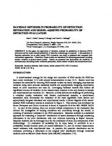
In the following section, the issue of interpolation where only three points are available is discussed. 2.2 Barycentric Interpolation Large aerodynamic and engine databases are used for the flight dynamic analysis. This data is accessed for analysis and synthesis tasks by table look up and linear interpolation. The reason for some of the data tables made available in the hypercube format is already discussed. The typical Mach number and AoA envelope is shown in Figure 3 where at higher Mach numbers limited range of angle of attack will be available.

Figure 3.

Angle of Attack – Mach number Envelope for a fighter aircraft (black vertical line indicates Mach number 1.0)

ISSN: 1694-2108 | Vol. 15, No. 3. MAY 2015

39

International Journal of Computer Science and Business Informatics

IJCSBI.ORG Table 1. 2D table as function of Mach number and Angle of Attack M => AOA -15.00 -14.00 -12.00 -10.00 -8.00 -6.00 -5.00 -4.00 -2.00 .00 2.00 4.00 6.00 8.00 10.00 11.00 12.00 13.00 14.00 15.00 16.00 17.00 18.00 19.00 20.00

.00 .2130 .2130 .2130 .2130 .2130 .2130 .2130 .2130 .2130 .2072 .2034 .2036 .2039 .2052 .2076 .2081 .2083 .2085 .2080 .2078 .2083 .2093 .2104 .2115 .2132

.

.30

.50

.60

.70

.80

.90

.95

1.00

1.05

1.10

1.20

.2130 .2130 .2130 .2130 .2130 .2130 .2130 .2130 .2130 .2072 .2034 .2036 .2039 .2052 .2076 .2081 .2083 .2085 .2080 .2078 .2083 .2093 .2104 .2115 .2132

.2019 2019 .2019 .2019 .2019 .2019 .2019 .2019 .2019 .1965 .1940 .1920 .1892 .1894 .1927 .1930 .1931 .1927 .1910 .1895 .1879 .1877 .1904 .1948 .2011

.1877 .1877 .1877 .1877 .1877 .1877 .1877 .1877 .1877 .1822 .1810 .1797 .1761 .1755 .1783 .1783 .1783 .1790 .1787 .1778 .1758 .1756 .1783 .1831 .1899

.1883 .1883 .1883 .1883 .1883 .1883 .1883 .1883 .1883 .1826 .1814 .1799 .1763 .1757 .1784 .1781 .1784 .1788 .1787 .1782 .1771 .1770 .1794 .1849 .1918

.1500 .1510 .1524 . .1539 .1543 .1543 .1530 .1532 .1509 .1490 .1447 .1402 .1382 .1384 .1387 .1333 .1314 .1316 .1352 .1394 .1447 .1483 .1506

.1508 1508 .1508 .1508 .1508 . .1508 .1514 .1502 .1465 .1397 .1324 .1300 .1315 .1323 .1303 .1256 .1223 .1203 .1221 .1250 .1284 .1288

.1628 .1628 .1628 .1628 1628 .1628 .1618 .1599 .1573 .1514 .1435 .1358 .1332 .1301 .1255 .1200 .1172 .1160 .1172 .1189 .1199 .1179

.1610 .1610 .1610 .1610 .1610 .1610 .1657 .1689 .1655 .1547 .1418 .1330 .1310 .1292 .1273 .1222 .1150 .1107 .1101 .1107 .1104 .1094

.1819 .1819 .1819 .1819 .1819 .1819 .1849 .1816 .1734 .1649 .1554 .1486 .1486 .1513 .1528 .1493 .1398 .1294 .1220 .1163 .1128 .1104

.1700 .1700 .1700 .1700 . .1700 .1700 .1699 .1659 .1586 .1510 .1438 .1408 .1420 .1444 .1442 .1391 .1294 .1200 .1156 .1136 .1125 .1104

.1443 .1443 1443 .1443 .1443 .1382 .1320 .1270 .1223 .1199 .1202 .1220 .1238 .1244 .1213 .1134 .1037 .0979 .0961 .0986 .0950

ISSN: 1694-2108 | Vol. 15, No. 3. MAY 2015

40

International Journal of Computer Science and Business Informatics

IJCSBI.ORG 21.00 22.00 23.00 24.00 25.00 26.00 27.00 28.00 29.00 30.00 31.00 32.00 33.00

.2157 .2189 .2225 .2269 .2312 .2345 .2370 .2393 .2394 .2377 .2342 .2295 .2242

.2157 .2189 .2225 .2269 .2312 .2345 .2370 .2393 .2394 .2377 .2342 .2295 .2242

.2079 .2158 .2227 .2285 .2345 .2384 .2386 .2356 .2292 .2237 .2210 .2171 .2297

.1967 .2034 .2088 .2139 .2208 .2269 .2299 .2305 .2288 .2252 .2222 .2183 .2277

.1987 .2035 .2052 .2087 .2179 .2281 .2341 .2364 .2380 .2271

.1527 .1587 .1654 .1655 .1612 .1573 .1575 .1537 .1467 .1334

ISSN: 1694-2108 | Vol. 15, No. 3. MAY 2015

.1283 .1245 .1213 .1171 .1138 .1122 .1143 .1191

41

.1155 .1120 .1107 .1113 .1137 .1144 .1120 .1102

.1081 .1067 .1045 .1029 .1050

.1093 .1081 .1051 .1075

.1093 .1108 .1103

International Journal of Computer Science and Business Informatics

IJCSBI.ORG

Accordingly, from Table 1, it is observed that at the areas marked with ovals only three points available for interpolation instead of conventional four points. To address this issue, we used Barycentric interpolation this facilitates full coverage of the aerodynamic database. Given a point r which lies within a triangle bounded by three vertices ( r1 , r2 , r3 ) in the plane, the barycentric weights ( 1 , 2 , 3 ) for each vertex respectively are given by (Wikepedia, 2014): 1

 1   ( x1  x3 ) ( x 2  x3 )   ( x  x3 )      ( y  y ) ( y  y )  ( y  y )  3 2 3   3   2  1 3  1  1  2

where, r1  ( x1 , y1 ), r2  ( x2 , y2 ), r3  ( x3 , y3 ), r  ( x, y)

If the function values at the three vertices ( r1 , r2 , r3 ) are given by the scalars ( z1 , z 2 , z 3 ) respectively, then the linearly interpolated value at point r is given by: 3

z   i z i i 1

It is noted that the weights ( 1 , 2 , 3 ) are all greater than zero if the point r lies within the triangle. If the point lies on the edge, the weight of the opposite vertex is zero. 3. RESULTS As discussed already, with the approximate trim calculations used as initial guess values for conventional optimization methods we can have faster convergence. Accordingly, a study is carried out for different flight conditions within the flight envelope for a level flight. The results are tabulated and presented in Table 2.

ISSN: 1694-2108 | Vol. 15, No. 3. MAY 2015

42

International Journal of Computer Science and Business Informatics

IJCSBI.ORG Table 2. Comparison of trim without and with Approximate Trim Calculations

Sl No. Case

Conventional Optimization method

1 2 3 4 5

198 163 86 43 47

0.3100M and 7.7374 km 0.4881M and 12.198 km 0.4000M and 4.572 km 0.7889M and 9.6387 km 1.2458M and 9.6387 km

Conventional Optimization method with approximate trim calculations 10 11 17 15 24

With the Barycentric interpolation, it is possible to cover full aerodynamic database with respect to Figure 3. 4. CONCLUSIONS For the nonlinear flight dynamic analysis and flight controller design, hundreds of linearised aircraft mathematical models are required. Aircraft trim is obtained by using the conventional numerical optimization methods. Approximate trim calculations are used to provide good initial guess values for the optimization methods for faster convergence. This also ensures global convergence within the flight envelope for the generation of equilibrium points. Similarly, for the cases at extreme pockets of the aerodynamic database where only three points are available for interpolation, we have used the Barycentric or triangular interpolation. Employing approximate trim calculations for optimization methods and Barycentric interpolation result in a computationally efficient nonlinear flight dynamic analysis and flight controller design with full coverage of aerodynamic database. REFERENCES [1] A. A. Pashilkar and S. Pradeep, 1999. Unsteady Aerodynamic modeling using Multivariate Orthogonal Polynomials. In: AIAA Atmospheric Flight Mechanics Conference and Exhibit. Portland, OR, August 9th – 11th, 1999. Reston: AIAA Publications [2] Brian L. Stevens and Frank L. Lewis, 1992. Aircraft Control and Simulation. New York: John Wiley & Sons Inc. [3] D. J. Bugajski and D. F. Enns, 1992. Nonlinear control law with application to high angle-of-attack flight. AIAA Journal of Guidance, Control, and Dynamics, 15(3), p 761-767. [4] David Allerton, 2009. Principles of Flight Simulation. Great Britain: Wiley Publications. [5] Eugene A. Morelli, 1995. Global Nonlinear Aerodynamic Modeling using multivariate orthogonal functions. AIAA Journal of Aircraft. 32 (2), p270-277

ISSN: 1694-2108 | Vol. 15, No. 3. MAY 2015

43

International Journal of Computer Science and Business Informatics

IJCSBI.ORG [6] Eugene A. Morelli, 1998. Global Nonlinear Parametric Modeling with Application to F-16 Aerodynamics. In: American Control Conference. Philadalphia, Pennsylvania, June 24-28, 1998. Piscataway, New Jersey: IEEE Publications [7] http://en.wikipedia.org/wiki/Barycentric_coordinate_system, accessed on 23rd June 2014. [8] J. M. Rolfe and K. J. Staples eds., 1991. Flight Simulation. New York: Cambridge University Press. [9] Mcruer D.T., Ashkenas I. and Graham D., 1973. Aircraft Dynamics and Automatic Control. Princeton: Princeton University Press. [10] Nandan K. Sinha and N.Ananthkrishnan, 2013. Elementary Flight Dynamics with an Introduction to Bifurcation and Continuation methods. New York: CRC Press [11] Shyam Chetty, Girish Deodhare and B. B. Misra, 2002. Design, development and flight testing of control law for the Indian Light Combat Aircraft. In:AIAA Guidance Navigation and Control Conference and Exhibit. Monterey, CA, August 5th – 8th, 2002. Reston: AIAA Publications

This paper may be cited as: Lathasree, P. and Pashilkar, A. A., 2015. Efficient Computational Tools For Nonlinear Flight Dynamic Analysis In The Full Envelope. International Journal of Computer Science and Business Informatics, Vol. 15, No. 3, pp. 26-44.

ISSN: 1694-2108 | Vol. 15, No. 3. MAY 2015

44