Received December 10, 2018, accepted December 28, 2018, date of current version January 29, 2019. Digital Object Identifier 10.1109/ACCESS.2019.2891699
Uncertainty-Aware Computational Tools for Power Distribution Networks Including Electrical Vehicle Charging and Load Profiles GIAMBATTISTA GRUOSSO 1 , (Senior Member, IEEE), GIANCARLO STORTI GAJANI1 , (Senior Member, IEEE), ZHENG ZHANG 2 , (Member, IEEE), LUCA DANIEL3 , (Senior Member, IEEE), AND PAOLO MAFFEZZONI 1 , (Senior Member, IEEE) 1 Politecnico
di Milano, Deib, 20133 Milan, Italy of Electrical and Computer Engineering, University of California at Santa Barbara, Santa Barbara, CA 93106, USA 3 Massachusetts Institute of Technology, Cambridge, MA 02139, USA 2 Department
Corresponding author: Giambattista Gruosso (
[email protected])
ABSTRACT As new services and business models are being associated with the power distribution network, it becomes of great importance to include load uncertainty in predictive computational tools. In this paper, an efficient uncertainty-aware load flow analysis is described which relies on generalized polynomial chaos and stochastic testing methods. It is described how the method can be implemented in order to account for real data-based load profiles due to two different usage models: residential loads and electrical vehicle charging profiles. Hence, it is shown how some relevant information affecting the quality of service can be deduced by means of non-elementary post-processing computations. The proposed technique is tested by using a benchmark scenario for typical European low voltage networks, considering the variation of both residential loads and EV charging profiles. The results are compared with the same simulation done by means of the Monte Carlo methodology. The consideration done during the analysis will be useful to clarify the application of the methodology but also to understand the effect of load variations on the grid characteristic quantities. INDEX TERMS Distribution network, load uncertainty, variability analysis, load forecasting, EV charging profiles, electrical vehicles.
I. INTRODUCTION
Electrical distribution networks are a specific kind of large scale systems that are designed to provide the required power to the loads while ensuring stability of node voltages, i.e. the quality of service. The recent trends towards the exploitation of renewable energy sources and the integration of new services, e.g. the charging of electrical vehicles, are introducing a remarkable variability of the powers that are delivered and/or absorbed at the terminal loads. Such a variability can jeopardize the stability of the network and the quality of service [1]. For such reasons, it is now noticeable the key role that uncertainty-aware computational tools can play during the design and real time control of power
VOLUME 7, 2019
distribution circuits [2]–[5]. In fact, such tools can provide a comprehensive view of the overall network: they can predict bus voltages and line currents variations at network points that can hardly be measured. The mainstream network uncertainty analysis approach adopts probabilistic models for the loads and uses repeatedly deterministic Load Flow (LF) analysis within a Monte Carlo (MC) iterative procedure. This approach, which is commonly referred to as Probabilistic Load Flow (PLF) analysis, can however be very time consuming and thus unpractical. Indeed, many open issues remain in PLF analysis. A first relevant issue is connected to modeling load uncertainty in a realistic way. Load modeling is commonly
2169-3536 2019 IEEE. Translations and content mining are permitted for academic research only. Personal use is also permitted, but republication/redistribution requires IEEE permission. See http://www.ieee.org/publications_standards/publications/rights/index.html for more information.
9357
G. Gruosso et al.: Uncertainty-Aware Computational Tools for Power Distribution Networks
based on statistical analyses of available customer profile data that are collected and analyzed for several network areas and utility types (e.g residential, commercial and industrial, electrical vehicles). Several modeling approaches exist, some of these are built on the aggregated data about the total load of the network, some others on the analysis of the statistical distribution of the loads at each node. In order to account for the interplay of many independent uncertain loads (i.e. variations in the active powers supplied at the different phases of the network) a great number of MC runs is needed to achieve a satisfactory statistical description. In fact, even though loads uncertainty can commonly be assumed to be Gaussian distributed, the nonlinear nature of load flow leads to state variable variations, e.g. maximum voltage at nodes or lines current, that are non-Gaussiandistributed. In this case, the statistical information about mean value and variance of an electric variable is not enough to describe it properly and the detailed Probability Density Function (PDF) shape is required for further inferences. The accurate determination of PDF with MC method can require tens of thousands repeated load flow analyses thus becoming very time consuming. To address the above issues, in this paper we focus on an efficient uncertainty quantification method recently presented in the literature [6], [7], and describe its specific application to the PLF problem [8], [9]. The method is based on generalized Polynomial Chaos (gPC) expansion and Stochastic Testing (ST) algorithm and is denoted as gPC+ST. Compared to other approximate techniques adopted for PLF analysis [2], [3], the gPC+ST method exhibits some features that make it well suitable for PLF applications. In fact, gPC+ST can be applied in connection to any available deterministic load flow solver without having to modify the codes. Furthermore, the gPC+ST method can deal with truly nonlinear problems that provide non-Gaussian-distributed output variables even in the case of uncertainty sources being modelled as Gaussian-distributed parameters. This is indeed the case for load flow analysis formulated in terms of node voltages and powers. As a first original contribution of this paper, we describe how the gPC+ST method can be implemented while accounting for real data-based load profiles. We will focus on two different types of load. The first is a mix of residential and commercial loads, while the second represents the power used to recharge electric vehicles.The two load categories are different one another, however, they are well suited to be interpreted in a unified probabilistic way. The profiles of the residential and commercial loads are considered from the low voltage side and the data are provided by the benchmark IEEE European low voltage test feeder network [10]. The benchmark is also used as a test network to demonstrate the validity of our method. The data relating to the recharging of electric vehicles, on the other hand, are measured and acquired in the context of the Italian project Teinvein [11] and represent a special case of recharging: low voltage and on recharging stations consisting 9358
of several parallel recharging points. These are used by a very specific fleet of vehicles that are the object of the cited project. A second contribution of our research is showing how the proposed method can be exploited to predict the detailed probability distribution and variability interval of a set of Quantities of Interest (QoI) that directly impact on the quality of service. Such variables can include the peak and minimum values assumed by the three phase voltages at some observable nodes as well as more general quantities that require non-elementary post-processing computations. In fact, real load profiles tend to produce sharp fluctuations in time of the node voltages. However, only the peak voltages that last for a sufficiently long period of time actually affect the quality of service. In this paper, we show how, for a given degree of variability of the load profiles, the proposed gPC+ST method can be exploited to deduce the probability that a node voltage will exceed a safe limit for a time duration W . The remainder of the paper is organized as follows: Sec. II reviews the deterministic load flow analysis; in Sec. III, we model load uncertainty and present the idea behind the gPC+ST method while in Sec. IV we provide the computational details. In Sec. V, we describe a relevant example of non-elementary post-processing computation and, finally, in Sec. VI we illustrate some application results in different scenarios. II. LOAD FLOW ANALYSIS
An electrical distribution system can be seen as a set of buses connected to each other by lines. Devices and equipment capable of providing or absorbing active and reactive power are connected to each one of the buses. The load flow problem consists in finding the set of voltages, i.e. the magnitude and angle, which, together with the network impedances, produces the load flows that are known to be correct at the system terminals. Assuming that the network is made of N buses and Nl lines, the problem is formulated mathematically as a set of nonlinear equations [12], [13] of the type: E = Sn − Vn Fn (V)
N X
Yni V∗i = 0
(1)
i=1
for n = 1, . . . , N . In (1), Sn = Pn + jQn denotes the complex power at node n where Pn and Qn are the active and reactive powers respectively, Vn is the node voltage phasor, while Yni are the entries of the bus admittance matrix. Node voltage E phasors are collected into vector V. Network terminations are specified by imposing the known active and reactive powers Pn , Qn absorbed or delivered by loads. Load conditions vary in time and thus the associated powers become functions of time, Pn (t), Qn (t). Let us consider a given observation time period (e.g. a day or a week), that is discretized into a sequence of Nt equally-spaced time instants tm = m · 1t, over which the load profiles are given. Node voltage waveforms Vn (t) are calculated by repeatedly solving the nonlinear problem (1) over the sequence of VOLUME 7, 2019
G. Gruosso et al.: Uncertainty-Aware Computational Tools for Power Distribution Networks
time instants tm . In doing that, the network state computed at time tm is used as the solver initial condition at next time tm+1 . III. UNCERTAINTY QUANTIFICATION WITH GENERALIZED POLYNOMIAL CHAOS A. MODELING LOAD VARIABILITY
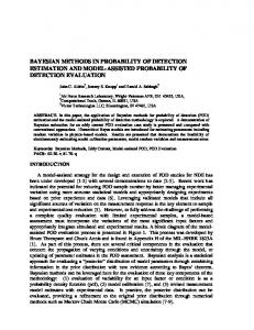
In the literature, load modeling is commonly achieved by exploiting historic data sets that are collected and analyzed for several network areas and utility types (e.g residential, commercial and industrial, electrical vehicles). Coherently with such an approach, the gPC-based methodology that we illustrate in this paper allows accounting for the typical time evolution (i.e. the chronological variation) of the most common power load profiles. The first type of loads herein considered are residential and commercial ones: these are single-phase loads connected at different nodes of the network. To realistically reproduce the effects that these loads could have on the network, we consider 55 different power profiles pRC n (t), with n = 1, . . . 55, selected among the ones provided with the benchmark test case [10]. These data represent with good approximation what can happen in a daily scenario. The 55 profiles are randomly subdivided into three roughly equivalent sets, and each set is then connected to one of the three phase lines (each load is connected to a different node). Fig. 1 shows the average value (i.e., the ensemble average) and the variability range of the loads for each phase line. It is evident how residential and commercial power demand is higher over certain time slots of the day where it can exhibit significant variability. In order to reproduce the uncertainty of the total power demand at each phase line the active power at the nth node is written as: h i RC Pn (t) = pRC (t) 1 + σ ξ j n n
FIGURE 1. Load variability in the three phases for the residential and commercial loads. The blue line present the mean value and the shadowed region the variability range. VOLUME 7, 2019
(2)
where we remind that pRC n (t) is the (known) nominal power profile over the time period. In (2), ξj denotes a zero-mean Gaussian-distributed statistical variable having unitary variance, i.e. hξj i = 0 and hξj2 i = 1, while σnRC is a scaling constant that determines the degree of variability.
FIGURE 2. Load variability in the three phases for the Electrical Vehicle Charging Stations. The blue line present the mean value and the shadowed region the variability range.
The second type of loads that we consider in this paper is the active power absorbed by EV charging stations. Fig. 2 shows some typical time evolutions of the EV power profiles pEV (t) measured during the research activity of the Italian Project TEINVEIN [11]. The electric vehicles that are considered in this project compose the fleet of a very successful urban car sharing service. These vehicles are recharged by service personnel at times of day with a distribution that is essentially optimized for the car sharing purposes: i.e. having the maximum number of charged vehicles at peak usage times. Similarly to what has been done for commercial and residential profiles, the EV profiles are randomly grouped into three sets and connected to the three phase lines. To the aim of reproducing the effect of EV loads and their statistical uncertainty, a second active power contribution h i P0n (t) = pEV (t) 1 + σnEV ξj (3) is added at the nth node, where σnEV is the degree of variability for the EV profile. Compared to the first type of loads, EV profiles exhibit some different features: they are more continuous with time and involve higher power consumptions. The addition of EV profiles thus enriches the scenario of the probabilistic analysis. We finally remark that the number of statistical parameters ξj employed does not necessarily corresponds to the number of nodes or loads, in fact sets of power profiles at different nodes can be scaled by the same statistical parameter. As an instance, in Sec. VI, devoted to applications, we will consider only three statistical ξj variables, one for each phase line. 9359
G. Gruosso et al.: Uncertainty-Aware Computational Tools for Power Distribution Networks
B. GENERALIZED POLYNOMIAL CHAOS
IV. COMPUTING THE GPC COEFFICIENTS
We consider a probabilistic problem where the uncertainty in the load power profiles is described by means of l stochastic parameters ξr modeling active power variability as in (2). Stochastic parameters are collected in the vector ξE = [ξ1 , ξ2 , . . . , ξl ]. The gPC method consists in adopting generalized polynomial chaos expansions for the node voltages. Depending on the numerical technique used to solve the gPC problem, the variables that have to be expanded can be all of the node voltages in the network or a subset of them, obviously these voltages are in general represented as complex phasors including magnitude and phase information. In some cases, the variables that we need to expand are limited to the quantities that we want to monitor: they may be the magnitude of some node voltages or line currents at a given time or the peak or minimum value assumed over a time period. In what follows, we will generically denote as V (t, ξE ) one of these variables. Under the mild hypothesis that V (t, ξE ) has finite variance (i.e. it is a second-order stochastic process), it can be approximated by an order-β truncated series [14]
There are two different mainstream approaches for computing the gPC expansion coefficients in (4): Galerkin Projection and Collocation Method [15].
V (t, ξE ) ≈
Nb X
ci (t) Hi (ξE ),
(4)
i=1
formed by Nb multi-variate basis functions Hi (ξE ) weighted by unknown polynomial chaos coefficients ci (t). The main feature in expression (4) is that the dependence of V (·) on the deterministic variable time, which is incorporated into coefficients ci (t), is separated by its dependence on statistical parameters ξE represented by basis functions Hi (ξE ). Each multi-variate basis function is given by the product Hi (ξE ) =
l Y
φir (ξr )
(5)
r=1
where φir (ξr ) is a univariate orthogonal polynomial of degree ir whose form depends on the density function of the rth parameter ξr . For instance, φir (ξr ) are Hermite polynomials if ξr is a Gaussian-distributed variable, while φir (ξr ) are Legendre polynomials if ξr is a uniformly distributed variable. A complete list of correspondence between several typical stochastic distributions and associated orthogonal polynomials can be found in [14]. For a given number of parameters l and series expansion truncation order β, the degrees ir of univariate polynomials in (5) forming Hi (ξE ), for r = 1, . . . , l, satisfy the following relation l X
ir ≤ β.
(6)
r=1
For generic truncation order β and number of parameters l, the number of gPC basis functions is given by [6] Nb = 9360
(β + l)! . β! l!
(7)
A. GALERKIN PROJECTION (GP)
Galerkin projection is an intrusive numerical technique that requires modifying the LF code (1). In accordance with the this method, a gPC expansion of the type (4) is adopted for each unknown nodal voltage Vn (t), i.e. Vn (t, ξE ) ≈
Nb X
cni (t) Hi (ξE ),
(8)
i=1
leading to Nb × N unknown cni coefficients that are complex variables. Such coefficients are determined by plugging the expansions (8) into (1) and then projecting the resulting nodal equations along the Nb basis functions. This results in a very large nonlinear system of size Nb × N , i.e. E ξE ), Hi (ξE )i = 0, hFn (V(
(9)
for n = 1, . . . , N and i = 1, . . . , Nb , where h·i denotes the inner product in the stochastic space [6]. The solution of (9) requires a significant computational effort both in terms of time and allocated memory. As an example, consider the case of a distribution network with N = 100 nodes, and suppose to perform stochastic Galerkin with l = 3 statistical parameters and expansion order β = 3. In this case, Nb = 20, so that the nonlinear system to be solved has size Nb × N = 2, 000. Due to problem nonlinearity, equations (9) tend to be strongly coupled among them (i.e. intermodulation of expansion coefficients) so that the computational time required for solving the system tends to grow as a power of two of the system size, i.e. about (Nb × N )2 . In our example, the computational time for solving the Galerkin problem is about 400× longer than that needed for a single LF analysis. The GP computational time grows very rapidly with the number of statistical parameters thus limiting the applicability of the method to networks of small size. B. STOCHASTIC COLLOCATION (SC)
SC is a nonintrusive method that can be combined with any LF formulation (1) without modifying the implementation codes. A second advantage of the SC method is that gPC expansion (4) is adopted limitedly to the set of network variables that we want to evaluate, i.e. the peak value of some monitoring node voltages. In what follows, we will focus on a recently proposed efficient implementation of SC method referred to as Stochastic Testing (ST) method. In accordance with the collocation-based Stochastic Testing (ST) [6], the Nb unknown coefficients cj (t) in the series (4) are calculated by properly selecting Ns = Nb testing points ξE k , for k = 1, . . . , Ns in the stochastic space where Vk (t) = V (t, ξE k ) is calculated with a deterministic LF analysis. VOLUME 7, 2019
G. Gruosso et al.: Uncertainty-Aware Computational Tools for Power Distribution Networks
At each testing point, the series expansion (4) is enforced to fit exactly (i.e., the polynomials interpolate the samples) the values Vk (t). Mathematically, this results in the following linear system M Ec(t) = VE (t),
(10)
where Ec(t) = [c1 (t), . . . , cNb (t)]T and VE (t) = [V1 (t), . . . , VNs (t)]T are the column vectors collecting the unknown coefficients and node voltage values respectively. The Nb × Nb square matrix M = {ak,i } = {Hi (ξE k )} collects the gPC basis functions evaluated at the testing points, i.e. H1 (ξE 1 ) ... HNb (ξE 1 ) .. .. .. M= (11) . . . . H1 (ξE Ns ) . . . HNb (ξE Ns ) It is worth noting that matrix M only depends on the selected basis functions and testing points, so that it can be precalculated, inverted and used for any t = tm as follows: Ec(tm ) = M−1 VE (tm ).
(12)
The ST method enables handling PLF problems with larger size and larger number of parameters. The selection of the testing points ξE k in the stochastic space is done so to ensure the highest numerical accuracy of the gPC-based interpolation scheme and of the associated statistical description. This is achieved by considering as testing points the (β + 1)l Gauss quadrature nodes in the l-dimensional stochastic space. Since the number (β + 1)l of nodes is greater than the number Nb of basis functions defined in (7), a subset formed by Ns = Nb quadrature nodes has to be selected as testing points in order to make problem (12) well posed. A possible method for selecting the subset of testing points among the quadrature nodes is presented in [6]. V. NON-ELEMENTARY POST-PROCESSING COMPUTATION
Once the coefficients cj (t) are computed, the mean value and standard deviation of an observable variable V (t, ξE ) can easily be determined [6]. Furthermore, and even more importantly, the gPC expansion (4) provides a compact model for the V (t, ξE ) multi-dimensional dependence. This enables repeated evaluations of V (t, ξE ) for large numbers of uncertainty vector realizations ξE k in very short times (one million evaluations require only few seconds on a quad-core computer) and the determination of the detailed shape of the PDF. Such accurately-computed PDF can then be exploited in further inferences such as the evaluation of the variability interval of the observable variable (with a certain confidence degree). More general information can further be deduced through non-elementary post-processing computations. In what follows, we illustrate two examples of non-elementary computing that are relevant for PLF applications. VOLUME 7, 2019
A. PEAK VOLTAGE LASTING FOR A TIME DURATION W
In this first example, we focus on the determination of the probability that a node voltage will exceed a safe limit VL for a time duration W . To this aim, and using the notation introduced in Sec. II, we consider the generic time window of duration W = nw 1t (with nw