The 2nd Joint International Conference on Multibody System Dynamics May 29–June 1, 2012, Stuttgart, Germany
Efficient Constraint Modeling for Closed-Chain Dynamics Abhinandan Jain, Cory Crean, Calvin Kuo, Marco B. Quadrelli Jet Propulsion Laboratory, California Institute of Technology 4800 Oak Grove Drive Pasadena, CA 91109, USA [Abhi.Jain, marco, calvinku]@jpl.nasa.gov,
[email protected] ABSTRACT In this article, we study the algorithmic and performance implications of different hinge and closure constraint modeling choices for closed-chain dynamics. Options for handling restricted inter-body relative motion range from the use of minimal coordinate hinges, to non-minimal coordinate ones utilizing bilateral constraints. In general, the closed-chain system model can be decomposed into a tree-topology sub-system subject to a set of closure constraints. We study three approaches for modeling the dynamics of such systems and compare the computational performance of their corresponding algorithms. We observe that with the use of structure-based, low-order algorithms, hinge based modeling offers significantly better simulation performance over constraint based techniques. 1
INTRODUCTION
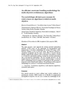
The subject of this paper is the dynamics of multibody systems with closed-loop topologies such as in Figure 1. The relative motion between adjacent bodies in a multibody system is constrained. Options for handling such inter-body constraints are to treat them as hinges, or as closure constraints between the bodies. In the hinge approach, the constraint is eliminated from the equations of motion by using minimal relative coordinates to parameterize the allowable motion between the body pair. On the other hand, the closure constraint approach employs non-minimal coordinates and utilizes bilateral constraints and Lagrange multipliers to enforce the restricted motion between body pairs. In this article, we study the algorithmic and performance implications of different hinge versus internal closed loop closure constraint modeling choices for closed-chain dynamics. While the use of hinges leads to equations of motion with smaller dimension, the accompanying minimal coordinates exhibit a high degree of dynamical coupling and a more complex formulation. However, the added complexity can be mitigated by the use of structure-based, low- Figure 1: A closed-chain multiorder, recursive methods for the dynamics computations. In contrast, body system with an internal the exclusive use of closure constraints leads to larger, but structurally closed loop constraint. simpler form of the equations of motion. More generally, closed-chain models contain a hybrid combination of hinges and closure constraints, with the hinges being associated with a tree topology sub-system within the overall model. We study the following three approaches for closed-chain dynamics that span the range of these modeling options: Fully-augmented (FA) method: The first method is the fully-augmented (FA) dynamics method [6, 13, 17]. In this method, all bodies are modeled as independent bodies using absolute coordinates, and the restricted relative motion is modeled via closure constraints as shown in Figure 2a. The advantage of this approach is that the equations of motion are simple and easy to set up. The mass matrix of the tree sub-system is block diagonal and constant. Sparse matrix solution techniques can be used to solve for Lagrange multiplier constraint forces. Disadvantages include the use of a large number of non-minimal generalized coordinates, the underlying differential-algebraic equation (DAE) structure of the equations of motion, and the need for error control techniques to manage constraint error growth during a simulation.
constraint aggregated body
constraints
(a) Fully augmented model
(b) Tree augmented model
(c) Constraint embedding model
Figure 2: In the fully augmented model (a), all bodies are treated as independent bodies with inter-body constraints. In the tree augmented model (b), the system is decomposed into a tree system together with a minimal set of inter-body constraints. In the constraint embedding model (c), internal loops are aggregated into bodies to convert the system into a tree topology system. Tree-augmented (TA) method: The second method is the tree-augmented (TA) dynamics method [9, 16]. In this method, a minimal set of the inter-body constraints are “cut” to obtain the tree-topology sub-system1 . The maximal spanning tree based tree sub-system only has hinges as illustrated in Figure 2b. The overall dynamics model consists of the minimal-coordinate dynamics model for the tree sub-system together with a minimal set of closure constraints. The number of generalized coordinates and closure constraints is much smaller compared with the FA model. The tree system’s mass matrix however is dense and configuration dependent, though low-order recursive algorithms are available for solving the tree system dynamics without requiring mass matrix inversion. The underlying formulation remains a DAE, but constraint error control is only needed for the smaller set of closure constraints. Constraint embedding (CE) method: The third method is the new constraint embedding (CE) dynamics method [10]. This technique uses the TA model as a starting point – where its closure constraints are eliminated by aggregating bodies affected by the closure constraint into compound bodies as shown in Figure 2c. The transformed system has a tree topology with only inter-body hinges and no closure constraints. The benefit of this minimal coordinates approach is that low-order tree algorithms can be directly used to solve the dynamics. Also, this formulation results in an ordinary differential equation (ODE) instead of a DAE, and constraint error control techniques are not required. This method however is more complex to implement, since the aggregated bodies now contain multiple rigid bodies and have configuration dependent geometry. While CE method shares the minimal coordinates attribute with projection dynamics techniques [6, 17], its advantage lies in the preservation of the system’s tree topology that is necessary for the use of the structure-based tree algorithms. This paper includes a brief overview of the analytical theory for solving closed-chain system dynamics using these approaches. In particular, we emphasize the use of structure-based, low-order recursive algorithms for solving the tree sub-systems dynamics and for solving for the constraint forces. Simulations of several small systems are used to cross validate the dynamics solutions from these three methods. A larger system consisting of a six-wheeled vehicle with wishbone suspensions at each of the wheels is used to compare the computational performance of these methods. Simulation runs for this system are carried out and the growth rate of the constraint and fidelity error is compared for different integration time steps across the methods. We hope that these results will help guide analysts in the judicious selection of dynamics modeling approaches and structure-based algorithms for closed chain dynamics simulations. 2
DYNAMICS WITH LOOP CONSTRAINTS
As we have seen, each of the FA, TA and CE models consist of a tree topology sub-system subject to a set of closure constraints. The specific details of the decomposition varies with the model type. For the FA model, 1 The
cuts and the spanning tree are non-unique in general.
the tree system is simply a collection of independent bodies, while the set of closure constraints is large. The CE model represents the other extreme, where the entire model is a tree topology system, and there are no additional closure constraints. The TA model is a hybrid, with a maximal spanning tree based tree topology system, together with a minimal set of closure constraints. In this section we study the general approach to solving the closed-chain equations of motion for such models consisting of tree topology systems with closure constraints. Using N to denote the number of degrees of freedom for the tree sub-system, the minimal coordinates equations of motion for the tree-topology sub-system can be expressed as M(θ) θ¨ + C(θ, θ˙ ) = T
(1)
where the configuration dependent, symmetric matrix M(θ) ∈ RN×N is the mass matrix of the system, C(θ, θ˙ ) ∈ RN denotes the velocity dependent Coriolis and gyroscopic forces vector, and T ∈ RN denotes the applied generalized forces. The mass matrix is positive-definite and invertible for tree-topology systems. Let nc denote the dimensionality of the closure constraints on the system, Then there exists a Gc (θ, t) ∈ Rnc ×N matrix and a U(t) ∈ Rnc vector that defines the velocity domain constraint equation for the holonomic and non-holonomic closure constraints on the system as follows: Gc (θ, t) θ˙ = U(t)
(2)
This differential form of the constraints is also referred to as a Pfaffian form. We assume that Gc (θ, t) is a full-rank matrix. Observe that Eq. 2 is linear in the θ˙ generalized velocity coordinates. These constraints effectively reduce the independent generalized velocities for the system from N to an (N − nc ) dimensional linear space, The dynamics of closed-chain systems can be obtained by modifying the tree system dynamics in Eq. 1 to include the effect of the closure constraints via Lagrange multipliers, λ ∈ Rnc , as follows2 M(θ) θ¨ + C(θ, θ˙ ) − G∗c (θ, t)λ = T Gc (θ, t) θ˙ = U(t)
(3)
The −G∗c (θ, t)λ term in the first equation represents the internal generalized constraint forces from the closure constraints. By differentiating the constraint equation, Eq. 3 can be rearranged into the following descriptor form: � �� � � � M G∗c θ¨ T−C � ˙ (t) − G ˙ c θ˙ ∈ Rnc = where U´ = U ´ −λ U Gc 0
(4)
One approach to solving the closed-chain dynamics equations of motion is to assemble the matrix on the left and the vector on the right in Eq. 4 and solve the linear matrix equation for the θ¨ generalized accelerations. This is especially attractive for the FA model, since the M matrix for this case is block diagonal and constant. Indeed, the whole matrix is highly sparse for this case. This approach is analyzed in detail in reference [17]. We on the other hand pursue an alternative Schur complement-based solution approach for the FA and TA models as described in the following lemma. Lemma 1. Augmented closed-chain forward dynamics solution The closed-chain dynamics generalized accelerations in Eq. 4 can be expressed as θ¨ = θ¨ f + θ¨ δ
(5)
where, the free generalized accelerations, θ¨ f , the correction generalized accelerations, θ¨ δ , and the Lagrange multipliers, λ, are given by θ¨ f
2 For
�
=
λ
=
θ¨ δ
=
�
M−1 (T − C) �−1 � − Gc M−1 G∗c γ M−1 G∗c λ
a matrix A, the A∗ notation denotes its matrix transpose.
(6a) where
γ = Gc θ¨ f − U´ �
(6b) (6c)
Proof. See [9, 15]. The θ¨ f = M−1 (T − C) term represents the generalized accelerations solution for the dynamics of the tree system while ignoring the closure constraints and, is therefore referred to as the free generalized accelerations. γ represents the acceleration-level constraint violation resulting from just the free dynamics of the system. The Gc M−1 G∗c matrix in Eq. 6b is the Schur complement of the matrix on the left hand side of Eq. 4. An intuitive interpretation of Eq. 6b is that the constraint error spatial accelerations from the free-dynamics solution, together with the Schur complement matrix allow the computation of the constraint forces necessary to nullify the errors. Once the constraint forces are available, Eq. 6c uses them to obtain the generalized accelerations to correct the free system dynamics solution. In summary, the solution to the closed-chain forward dynamics thus conceptually involves the following steps: 1. Solve Eq. 6a for the θ¨ f free generalized accelerations. 2. Use θ¨ f and the Gc M−1 G∗c Schur complement to solve for the λ Lagrange multipliers via Eq. 6b. 3. Use λ to solve Eq. 6c for the θ¨ δ correction accelerations, 4. Compute the θ¨ generalized accelerations using Eq. 5. Only the first step is needed when closure constraints are absent. One numerical consequence of the use of non-minimal coordinates and closure constraints is that differential-algebraic equation (DAE) integrators, instead of the ODE integrators for tree systems, are required for the numerical integration of the accelerations and velocities [1, 17]. Furthermore, error control techniques are needed to manage the growth of constraint errors that can cause the system state to drift off of the constraint manifold [2, 3, 17]. 3
COMPUTATIONAL ALGORITHMS
The solution for the closed-chain equations of motion requires a step for solving the tree system equations of motion, followed by solving for the constraint forces from the closure constraints, and finally a step to correct for the effect of these correction forces. In this section we describe analytical results and structurebased, low order computational algorithms for the key computationally demanding steps. 3.1 Tree Topology Dynamics Using spatial operators one can obtain operator factorizations of the tree topology mass matrix and its inverse as follows [9, 15]: M = HφMφ∗ H∗ = [I + HφK]D[I + HφK]∗ [I + HφK]−1 = I − HψK
(7)
M−1 = [I − HψK]∗ D−1 [I − HψK] The first expression defines the Newton-Euler operator factorization of the mass matrix M in terms of the H hinge articulation, the φ rigid body propagation and the M link spatial inertia operators [8, 9]. While this factorization has non-square factors, the second expression describes an alternative factorization involving only square factors with block diagonal D and block lower-triangular [I + HφK] matrices. . The next expression describes an analytical expression for the inverse of the [I + HφK] operator. Using this equation leads to the final analytical expression for the inverse of the mass matrix. These operator expressions hold generally for tree-topology systems irrespective of the number of bodies, the types of hinges, the specific topological structure and even for the case of non-rigid links [9]. The spatial operators ψ, D correspond to a suitably defined spatially recursive Kalman filter, with the spatial operator K representing the Kalman gain for this filter. We also refer to these operators ψ, D and K as"articulated" quantities, because of their relationship to the articulated inertias first introduced by [4].
Using the expression for the mass matrix inverse in Eq. 7, and some additional spatial operator identities, it can be shown that [7] 7 1 θ¨ = M−1 (T − C) = [I − HψK]∗ D−1 [I − HψK](T − C) � � = [I − HψK]∗ D−1 T − Hψ[KT + Pa + b] − K∗ ψ∗ a
(8)
The articulated body (AB) forward dynamics algorithm is a well known structure-based O(N) procedure for evaluating θ¨ in Eq. 8 [5, 9]. The algorithm consists of multiple recursive sweeps across the tree links. This tree forward dynamics algorithm does not require the explicit computation of either M or C or of any of the spatial operators. 3.2 Closed-Chain Dynamics with Loop Constraints Let us assume that the closed-chain constraints are loop constraints on the spatial velocities of a set of closure nodes. Let Vnd denote the spatial velocities of these closure nodes. Then for some matrix Q that describes the geometric nature of the closures, the closure constraints (holonomic or non-holonomic) can be expressed as QVnd − U = QJ θ˙ − U = 0 (9) with J denoting the velocity Jacobian matrix for these constraint nodes on the system. Using Eq. 2 and the J = B∗ φ∗ H∗ operator expression3 for the Jacobian matrix [9], we can identify Gc as Gc = QJ = QB∗ φ∗ H∗
(10)
This specific form for Gc allows us to simplify the expressions in Lemma 1, as described in the following lemma. Lemma 2. Forward dynamics with loop constraints The generalized accelerations for a closed-chain system with loop constraints, given by Eq. 10, is θ¨ = θ¨ f + θ¨ δ
(11)
where, the free generalized accelerations, θ¨ f , the correction generalized accelerations, θ¨ δ , and the Lagrange multipliers, λ, are given by θ¨ f
�
=
� � [I − HψK]∗ D−1 T − Hψ[KT + Pa + b] − K∗ ψ∗ a ∗ −1
where
λ
=
−[QΛQ ]
θ¨ δ
�
[I − HψK]∗ D−1 HψBQ∗ λ
=
γ
�
γ(θ, t) =
Qαfnd
˙ Vnd ˙ (t) + Q − U
(12a) (12b) (12c)
with αfnd denotes the spatial accelerations of the constraint nodes for the free-dynamics solution of Eq. 12a, �
�
and Λ = B∗ ΩB with Ω = ψ∗ H∗ D−1 ψH. Proof. See [9, 15]. This lemma provides explicit operator expressions for the constraint forces and the generalized accelerations which form the basis of structure-based, low-order computational algorithms for solving the closed-chain dynamics. We have already observed in section 3.1 that Eq. 12a can be evaluated using the low-order O(N) AB forward dynamics algorithm. In addition, Eq. 12b uses the QΛQ∗ expression for the Schur complement that unlike Eq. 6b does not require the the mass matrix inverse. Low-order algorithms for computing the Schur complement are discussed in section 3.3. The computational algorithms and steps for the solution of the closed-chain dynamics with loop constraints in Lemma 2 are summarized below: 1. Solve for θ¨ f in Eq. 12a using the O(N) AB forward dynamics algorithm. This also results in the computation of the articulated body inertia quantities and the αfnd node spatial accelerations required by Eq. 12b. 3B
is a pick-off operator defined in reference [9].
2. Compute Λ using the procedure in section 3.3 and solve the Eq. 12b matrix equation for the λ Lagrange multipliers. 3. Use the O(N) AB algorithm to compute θ¨ δ = [I − HψK]∗ D−1 HψBQ∗ λ. 4. Use Eq. 11 to compute θ¨ . This procedure is of O(N) computational complexity, except for the step involving the solution of the Eq. 12b matrix equation which can be cubic in the number of constraints. This procedure is directly applicable to solving the closed-chain dynamics equations of motion using either of the FA or TA models. The only difference between these methods is the specific nature of the tree sub-system and the set of closure constraints in the underlying models. The CE model on the other hand is a tree-topology system that does not include any closure constraints. This tree-topology model is obtained by aggregating the bodies associated with the closure constraints into variable geometry bodies. The aggregation process is carried out in a way such that the transformed system’s topology is that of a tree. The detailed description of the procedure for constraint embedding is described in [9, 10]. Due to the tree-topology structure of the resulting model, the solution to its equations of motion only requires the AB algorithm. Due to the more complex nature of the aggregated bodies, the recursive forward dynamics steps in processing these bodies are more expensive and the computational cost scales as the square of the number of combined degrees of freedom for the bodies within the aggregated bodies. 3.3 Schur Complement Matrix Computation Even though the mass matrix inverse is no longer needed, one of the computational bottlenecks in the procedure described above, is the evaluation of the Λ Schur complement matrix required for obtaining the constraint forces. The brute force evaluation of Ω and Λ = B∗ ΩB is computationally very expensive and scales as the cube of the number of degrees of freedom in the system. However, this Schur complement matrix is mathematically identical to the operational space inertia matrix used in robot system control [14] and structure-based, low-order algorithms for computing it have been developed using spatial operator techniques [9, 12, 16]. These algorithms exploit a decomposition of the Ω matrix into a disjoint sum of a diagonal, and upper and lower triangular matrices, and a highly sparse matrix. This decomposition has the additional special property that all the matrices in the decomposition can be derived from the diagonal matrix. The overall computational complexity of this structure-based algorithm is just quadratic in nc . 4
NUMERICAL VALIDATION
We have used simulations for the following standard closed-chain mechanisms [6] to cross-validate the FA, TA and CE dynamics solution techniques: 1. Planar crank slider mechanism: The planar crank slider mechanism (Figure 3a) is a 3 body system with 3 tree degrees of freedom and a single 1 degree of freedom closure loop constraint. The mechanism has single degree of freedom rotary and prismatic hinges.
(a) Planar Crank Slider
(b) Quick Return
(c) Planar Four Bar
(d) Spatial Four Bar
(e) Spatial Crank Slider
Figure 3: Closed-loop mechanisms used for cross-validating the FA, TA and CE dynamics algorithms.
(a) Planar Four Bar
(b) Spatial Crank Slider
Figure 4: Plots of generalized coordinate trajectories over time from simulation runs using the FA, TA and CE methods using 0.1ms integration time step. The plot on the left is for one of the angle coordinates for the planar four bar mechanism, while the one on the right is for the position of the slider for the spatial crank slider mechanism. The trajectories from the 3 methods are in close agreement and are hence indistinguishable in the plots. 2. Planar quick return mechanism: The planar quick return mechanism (Figure 3b) is a 5 body system with 5 tree degrees of freedom and two 1 degree of freedom closure loop constraints. The mechanism has single degree of freedom rotary and prismatic hinges. 3. Planar four-bar mechanism: The planar four-bar mechanism (Figure 3c) is a 4 body system with 3 tree degrees of freedom and a single 1 degree of freedom closure loop constraint. The mechanism has single degree of freedom rotary hinges. 4. Spatial four-bar mechanism: The spatial four-bar mechanism (Figure 3d) is a 4 body system with 4 tree degrees of freedom and a single 3 degree of freedom closure loop constraint. The mechanism has single degree of freedom rotary hinge, a 2 degree of freedom universal joint hinge and a 3 degree of freedom spherical joint. 5. Spatial crank slider mechanism: The spatial crank slider mechanism (Figure 3e) is a 4 body system with 6 tree degrees of freedom and a single 1 degree of freedom closure loop constraint. The mechanism has a single degree of freedom rotary and prismatic hinges and a 3 degree of freedom spherical joint. In each of these simulation examples, a steady torque is applied at one of the joints to drive the dynamics, and an explicit RK4 integrator is used to integrate the dynamics solution. Figure 3 shows example trajectory plots for the position of selected points on the mechanisms. The trajectories from all of the solution methods tracked each other closely and helped to cross-validate the solution methods. 5
COMPUTATIONAL PERFORMANCE
In this section we use simulations of NASA’s Lunar Electric Rover (LER) vehicle shown in Figure 5a to compare the computational performance of the three methods. The LER is a 6-wheeled rover, with each wheel mounted via an independent wishbone suspension consisting of a planar four-bar linkage. Overall, this larger vehicle model contains 31 bodies. The simulation model uses a free-floating model of the vehicle under a gravitational field. The wishbone suspensions are spring loaded to support the weight of the vehicle. In the simulation run, out of phase sinusoidal forces are applied to the wheels to mimic terrain interaction forces. The effect is to induce a periodic motion in each of the suspension elements and an overall rotation of the vehicle. Overall, eight different methods were used to carry out the simulation. Two of these were variants of the CE method, with one using an analytic solution for the four-bar linkage kinematics, while the other one used a numerical iterative procedure. Three variants of each of the TA and FA methods were used. One variant used no constraint error control, while the others used the Baumgarte and inverse kinematics (IK) based projection error control techniques [3]. Figure 5b shows the time trajectory of points on the vehicle from solving the dynamics using all the methods. The results from all of the methods showed good agreement.
(a) LER Vehicle
(b) LER Vehicle Positions
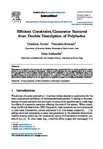
Figure 5: A simulation of the LER vehicle using the FA, TA and CE methods. The plot on the right shows the time history of the displacements of three points on the vehicle. The close agreement of the trajectories across the methods makes them indistinguishable in the plot. Figure 6 is a log-log scatter plot that compares the computational and numerical performance of the different methods for a 1s simulation of the vehicle using a fixed step, explicit RK4 integrator. Each of the points represents a different method and integration time step combination. The X axis displays the wall clock time for each of the methods. The Y axis for the left plot displays the constraint violation errors. It shows that the CE method has the best error and speed performance, followed by that of the TA method with the FA method showing a significant drop in computational speed for similar error performance. Also, as expected, the computational cost increases as the time step is decreased,and the inverse kinematics projection based constraint error control is somewhat more expensive than the Baumgarte method. The scatter plot on the right tells a similar story, except that the Y axis this time is a measure of the fidelity error. Simulation results from .01ms integration time step runs showed good agreement across the different methods, and were used as the baseline to compute the fidelity errors for the other runs. A simulation duration of 1s was used for these comparisons because longer simulation runs showed similar trends, but with increased failures from constraint error growth for the TA and FA methods. Table 1 summarizes the specific performance values for a 1ms integration time step simulations. Method CE (analytic) CE (non-analytic) TA (no error control) TA w/ Baumgarte TA w/ projection FA (no error control) FA w/ Baumgarte FA w/ projection
Tree dofs 24 24 36 36 36 186 186 186
Constraints size 0 0 12 12 12 162 162 162
Constraint error 1.3069e−31 3.7367e−15 5.2351e−13 1.3466e−13 5.2175e−13 2.4183e−09 5.7032e−11 Incomplete
Fidelity error 0.00563109 0.00563108 0.00563094 0.00563121 0.00999659 0.02183112 0.01082618 -
Normalized wall clock time 1.0000 1.7296 1.6007 1.6362 1.5907 59.4236 59.4648 -
Table 1: Model parameters for the FA, TA and CE methods for the LER vehicle simulation, together with a comparison of the constraint error, fidelity error and simulation wall clock time across the methods for a 1ms time step, 3s long simulation run.
6
CONCLUSIONS
In this article, we have studied and compared the performance of the FA, TA and CE approaches for solving closed-chain dynamics. While the TA and CE models are more complex, we have shown that the use of structure based recursive algorithms can be used to address the added complexity, while significantly improving computational and numerical performance. In particular, we have used the O(N) articulated body
(a) LER Constraint Errors Scatter Plot
(b) LER Fidelity Scatter Plot
Figure 6: Scatter plots comparing the performance of the FA, TA and CE techniques for simulating the dynamics of the LER vehicle. Three variants of the TA and FA methods were used: with no error control, with Baumgarte error control, and with inverse kinematics (IK) projection after each time step. Two variants of the CE method were used; with analytic and iterative solution of the four-bar kinematics. For each method, the simulation was run with time steps of 2ms, 1ms, .25ms, .1ms and 0.04ms, with the smaller symbols denoting smaller time steps. The plot on the left shows the average constraint violation error versus wall clock time for different methods. The figure on the right is a similar scatter plot but with the Y axis showing the fidelity error for each of the methods. Both plots show that reducing the time step reduced errors but increased the computational cost. The analytical CE method out performs the other methods, while the FA methods perform poorly compared to the others. forward dynamics algorithm for solving the tree-topology dynamics, along with the structure-based, loworder operational space inertia algorithm for computing the Schur complement matrix needed for computing the constraint forces. Numerical experiments to validate each of the methods show very good agreement across a variety of standard closed-chain mechanism problems. A larger 6-wheeled LER vehicle model was used for a detailed comparison of the performance of each of the methods. A comparison of the error performance and computational time across the methods showed the CE method as having the best performance, the FA method significantly worse performance, with the TA method being in the middle.These comparisons show that by taking advantage of structure-based low-order algorithms, the added complexity of the hinge-based methods is well rewarded by significantly superior performance over constraint-based methods. Similar formulation and performance issues have been examined for multibody systems with both closure constraints as well as contact (unilateral) constraints [11]. The system topology plays a significant role in the choosing between the CE and TA methods. The computational cost of the CE method is cubic in the number of degrees of freedom within the embedded loops. On the other hand, the computational cost of the TA method is cubic in the total number of closure constraints. Thus, the CE method is preferable for closed-chain systems with small size loops. On the other hand, the TA method is suitable for systems with a small number of large loops. In general, a hybrid combination of the TA and CE techniques will provide the optimal performance. In this approach, the small loops can be aggregated using the CE approach, while the large loops can be cut along the lines of the TA approach. In future work we plan to study such hybrid schemes, as well as simulation performance for a broader family of variable-step, implicit and DAE integrators.
Acknowledgments The research described in this paper was performed at the Jet Propulsion Laboratory (JPL), California Institute of Technology, under contract with the National Aeronautics and Space Administration.4 This project was also supported in part by Grant Number RO1GM082896-01A2 from the National Institute of Health. REFERENCES [1] A SCHER , U. M., AND P ETZOLD , L. R. Computer Methods for Ordinary Differential Equations and Differential-Algebraic Equations. SIAM, 1998. [2] BAUMGARTE , J. Stabilization of constraints and integrals of motion in dynamical systems. Comput. Methods Appl. Mech. Eng. 1 (1972), 1–16. [3] C HANG , C. O., AND N IKRAVESH , P. E. Optimal design of mechanical systems with constraint violation stabilization method. J. of Mechanisms, Transmissions, and Automation in Design 107 (Dec. 1985), 493–498. [4] F EATHERSTONE , R. The Calculation of Robot Dynamics using Articulated-Body Inertias. The International Journal of Robotics Research 2, 1 (1983), 13–30. [5] F EATHERSTONE , R. Rigid Body Dynamics Algorithms. Springer Verlag, 2008. [6] H AUG , E. J. Elements of Computer-Aided Kinematics and Dynamics of Mechanical Systems: Basic Methods. Springer-Verlag, 1984. [7] JAIN , A. Unified formulation of dynamics for serial rigid multibody systems. Journal of Guidance Control and Dynamics 14, 3 (Nov. 1991), 531–542. [8] JAIN , A. Graph Theoretic Foundations of Multibody Dynamics Part II: Analysis and Algorithms. Multibody System Dynamics 26, 3 (Oct. 2011), 335–365. [9] JAIN , A. Robot and Multibody Dynamics: Analysis and Algorithms. Springer, 2011. [10] JAIN , A. Multibody graph transformations and analysis Part II: Closed-chain constraint embedding. Nonlinear Dynamics 67, 3 (Aug. 2012), 2153–2170. [11] JAIN , A., C REAN , C., K U , C., VON B REMEN , H., AND M YINT, S. Minimal Coordinate Formulation of Contact Dynamics in Operational Space. In review. [12] K REUTZ -D ELGADO , K., JAIN , A., AND RODRIGUEZ , G. Recursive formulation of operational space control. The International Journal of Robotics Research 11, 4 (1992), 320–328. [13] O RLANDEA , N., C HACE , M. A., AND C ALAHAN , D. A. A Sparsity-Oriented Approach to the Dynamic Analysis and Design of Mechanical Systems - PART 1. ASME J. Engineering for Industry 99, 2 (1977), 773–779. [14] O USSAMA K HATIB. Object Manipulation in a Multi-Effector System. In 4th International Symposium on Robotics Research (Santa Cruz, CA, May 1988), pp. 137–144. [15] RODRIGUEZ , G., JAIN , A., AND K REUTZ -D ELGADO , K. A spatial operator algebra for manipulator modeling and control. The International Journal of Robotics Research 10, 4 (1991), 371. [16] RODRIGUEZ , G., JAIN , A., AND K REUTZ -D ELGADO , K. Spatial operator algebra for multibody system dynamics. Journal of the Astronautical Sciences 40, 1 (1992), 27–50. [17]
VON S CHWERIN , R. Springer, 1999.
4 �2012 c
Multibody system simulation: numerical methods, algorithms, and software.
California Institute of Technology. Government sponsorship acknowledged.