... data associ- ation problem is typically hard due to potential ambiguities ... constraints. To find the constraints from laser range data one ..... From these rotations, we recover the updated .... Again, we corrupted the observations with a variable ...
Non-linear Constraint Network Optimization for Efficient Map Learning Giorgio Grisetti∗
Cyrill Stachniss
Wolfram Burgard
University of Freiburg, Department of Computer Science, 79110 Freiburg, Germany {grisetti | stachnis | burgard}@informatik.uni-freiburg.de, ∗ corresponding author
Abstract— Learning models of the environment is one of the fundamental tasks of mobile robots since maps are needed for a wide range of robotic applications, such as navigation and transportation tasks, service robotic applications, and several others. In the past, numerous efficient approaches to map learning have been proposed. Most of them, however, assume that the robot lives on a plane. In this paper, we present a highly efficient maximum likelihood approach that is able to solve 3D as well as 2D problems. Our approach addresses the so-called graph-based formulation of the simultaneous localization and mapping (SLAM) and can be seen as an extension of Olson’s algorithm [27] towards non-flat environments. It applies a novel parameterization of the nodes of the graph that significantly improves the performance of the algorithm and can cope with arbitrary network topologies. The latter allows us to bound the complexity of the algorithm to the size of the mapped area and not to the length of the trajectory. Furthermore, our approach is able to appropriately distribute the roll, pitch and yaw error over a sequence of poses in 3D mapping problems. We implemented our technique and compared it to multiple other graph-based SLAM solutions. As we demonstrate in simulated and in real world experiments, our method converges faster than the other approaches and yields accurate maps of the environment.
I. I NTRODUCTION To efficiently solve the majority of robotic applications such as transportation tasks, search and rescue, or automated vacuum cleaning a map of the environment is required. Acquiring such models has therefore been a major research focus in the robotics community over the last decades. Learning maps under pose uncertainty is often referred to as the simultaneous localization and mapping (SLAM) problem. In the literature, a large variety of solutions to this problem can be found. The approaches mainly differ in the underlying estimation technique such as extended Kalman filters, information filters, particle filters, smoothing, or least-square error minimization techniques. In this paper, we consider the popular and so-called “graphbased” or “network-based” formulation of the SLAM problem in which the poses of the robot are modeled by nodes in a graph [5, 8, 11, 14, 16, 22, 27, 13, 36, 26]. Spatial constraints between poses that result from observations and from odometry are encoded in the edges between the nodes. In the context of graph-based SLAM, one typically considers two different problems. The first one is to identify the constraints based on sensor data. This so-called data association problem is typically hard due to potential ambiguities or symmetries in the environment. A solution to this problem is often referred to as the SLAM front-end and it directly
before optimization after optimization
Fig. 1. Constraint network corresponding to a dataset recorded with an instrumented car at the EPFL campus in Lausanne before (left) and after (right) optimization. The corrected network is overlayed with an aerial image.
deals with the sensor data. The second problem is to correct the poses of the robot to obtain a consistent map of the environment given the constraints. This part of the approach is often referred to as the optimizer or the SLAM back-end. To solve this problem, one seeks for a configuration of the nodes that maximizes the likelihood of the observations encoded in the constraints. Often, one refers to the negative observation likelihood as the error or the energy in the network. An alternative view to the problem is given by the spring-mass model in physics. In this view, the nodes are regarded as masses and the constraints as springs connected to the masses. The minimal energy configuration of the springs and masses describes a solution to the mapping problem. As a motivating example, Figure 1 depicts an uncorrected constraint network and the corresponding corrected one. Popular solutions to compute a network configuration that minimizes the error introduced by the constraints are iterative approaches. They can be used to either correct all poses simultaneously [14, 20, 22, 36] or to locally update parts of the network [5, 11, 13, 16, 26, 27]. Depending on the used technique, different parts of the network are updated in each iteration. The strategy for defining and performing these local updates has a significant impact on the convergence speed. In this paper, we restrict ourselves to the problem of finding the most likely configuration of the nodes given the constraints. To find the constraints from laser range data one can, for example, apply the front-end of the ATLAS framework introduced by Bosse et al. [2], hierarchical SLAM [6], or the work of N¨uchter et al. [26]. In the context of visual SLAM, a potential approach to obtain such constraints has recently
been proposed by Steder et al. [33]. Our approach uses a tree structure to define and efficiently update local regions in each iteration by applying a variant of stochastic gradient descent. It extends Olson’s algorithm [27] and converges significantly faster to highly accurate network configurations. Compared to other approaches to 3D mapping, our technique utilizes a more accurate way to distribute the rotational error over a sequence of poses. Furthermore, the complexity of our approach scales with the size of the environment and not with the length of the trajectory as it is the case for most alternative methods. The remainder of this paper is organized as follows. In Section II, we formally introduce the graph-based formulation of the mapping problem and explain the usage of stochastic gradient descent to reduce the error of the network configuration. Whereas Section III introduces our tree parameterization, Section IV describes our approach to distribute the rotational errors over a sequence of nodes. In Section V we then provide an upper bound for this error distribution. Section VI, explains how to obtain a reduced graph representation to limit the complexity. After describing the experimental results with our approach in Section VII, we provide a detailed discussion of related work in Section VIII. II. M AXIMUM L IKELIHOOD M APPING USING A C ONSTRAINT N ETWORK Most approaches to network-based or graph-based SLAM focus on estimating the most-likely configuration of the nodes and are therefore referred to as maximum-likelihood (ML) techniques [5, 11, 13, 14, 22, 27, 36]. Such techniques do not compute the full posterior about the map and the poses of the robot. The approach presented in this paper also belongs to this class of methods. A. Problem Formulation The goal of graph-based ML mapping algorithms is to find the configuration of the nodes that maximizes the likelihood of the observations. For a more precise formulation consider the following definitions: T • Let x = (x1 · · · xn ) be a vector of parameters which describes a configuration of the nodes. Note that the parameters xi do not need to be the absolute poses of the nodes. They are arbitrary variables which can be mapped to the poses of the nodes in real world coordinates. • Let us furthermore assume that δji describes a constraint between the nodes j and i. It refers to an observation of node j seen from node i. These constraints are the edges in the graph structure. • The uncertainty in δji is represented by the information matrix Ωji . • Finally, fji (x) is a function that computes a zero noise observation according to the current configuration of the nodes j and i. It returns an observation of node j seen from node i. Figure 2 illustrates an observation between two nodes. Given a constraint between node j and node i, we can define the error eji introduced by the constraint as eji (x)
= fji (x) − δji
(1)
Fig. 2.
Example of an observation of the node j seen from i.
as well as the residual rji rji (x)
= −eji (x).
(2)
Note that at the equilibrium point, eji is equal to 0 since fji (x) = δji . In this case, an observation perfectly matches the current configuration of the nodes. Assuming a Gaussian observation error, the corresponding negative log likelihood results in Fji (x)
T
∝ (fji (x) − δji ) Ωji (fji (x) − δji ) = eji (x)T Ωji eji (x)
(3) (4)
= rji (x)T Ωji rji (x).
(5)
Under the assumption that the observations are independent, the overall negative log likelihood of a configuration x is X F (x) = Fji (x) (6) hj,ii∈C
∝
X
rji (x)T Ωji rji (x).
(7)
hj,ii∈C
Here C = {hj1 , i1 i , . . . , hjM , iM i} is a set of pairs of indices for which a constraint δjm im exists. The goal of an ML approach is to find the configuration x∗ of the nodes that maximizes the likelihood of the observations. This can be written as x∗ = argmin F (x).
(8)
x
There are multiple ways of solving Eq. (8). They range from approaches applying gradient descent, conjugate gradients, Gauss Seidel relaxation, multi-level relaxation, or LUdecomposition. In the following section, we briefly introduce stochastic gradient descent, which is the technique our approach is based on. B. Stochastic Gradient Descent for Maximum Likelihood Mapping Olson et al. [27] propose to use a variant of the preconditioned stochastic gradient descent (SGD) to address the SLAM problem. The approach minimizes Eq. (8) by sequentially selecting a constraint hj, ii (without replacement) and by moving the nodes of the network in order to decrease the error introduced by the selected constraint. Compared to the standard formulation of gradient descent, the constraints are not optimized as a whole but individually. The nodes are updated according to the following equation: xt+1
T = xt + λ · KJji Ωji rji {z } | ∆xji
(9)
Here x is the set of variables describing the locations of the poses in the network and K is a pre-conditioning matrix. Jji is the Jacobian of fji , Ωji is the information matrix capturing the uncertainty of the observation, and rji is the residual. Reading the term ∆xji of Eq. (9) from right to left gives an intuition about the iterative procedure: • The term rji is the residual which corresponds to the negative error vector. Changing the network configuration in the direction of the residual rji will decrease the error eji . • The term Ωji represents the information matrix of a constraint. Multiplying it with rji scales the residual components according to the information encoded in the constraint. T • The Jacobian Jji maps the residual term into a set of variations in the parameter space. • The term K is a pre-conditioning matrix. It is used to scale the variations resulting from the Jacobian depending on the curvature of the error surface. Approaches such as Olson’s algorithm [27] or our previous work [13] apply a diagonal pre-conditioning matrix computed from the Hessian H as K
=
[diag(H)]−1 .
(10)
Finally, the quantity λ is a learning rate that decreases with each iteration of SGD and that ensures the convergence of the system. In practice, the algorithm decomposes the overall problem into many smaller problems by optimizing each constraint individually. Thus, a portion of the network, namely the nodes involved in a constraint, is updated in each step. Obviously, updating the different constraints one after each other can have antagonistic effects on a subset of variables. To merge the contribution of the individual constraints, one uses the learning rate to reduce the fraction of the residual which is used for updating the variables. This makes the solutions of the different sub-problems to asymptotically converge towards an equilibrium point that is the solution reported by the algorithm. Whereas this framework allows us to iteratively reduce the error given the network of constraints, it leaves open how the nodes are represented or parameterized. However, the choice of the parameterization has a strong influence on the performance of the algorithm. The next section addresses the problem of how to parameterize a graph so that the optimization can be carried out efficiently. •
III. T REE PARAMETERIZATION FOR SGD The poses p = {p1 , . . . , pn } of the nodes define the configuration of the network. They can be described by a vector of parameters x such that a bijective mapping g between p and x exists. x = g(p)
p = g −1 (x)
(11)
As explained above, in each iteration SGD decomposes the problem into a set of subproblems and solves them sequentially, where a subproblem is the optimization of a single constraint.
The parameterization g defines not only how the variables of the nodes are described but also the subset of variables that are modified by a single constraint update. A good parameterization defines the subproblems in a way that the combination step leads only to small changes of the individual solutions. Olson et al. [27] proposed to use the so-called incremental pose parameterization for 2D problems. For each node i in the graph, they store a the parameter xi which is the vector difference between the poses of the node i and the node i − 1 xi = pi − pi−1 .
(12)
This parameterization has the advantage of allowing fast constraint updates. As discussed in [13], updating a constraint between two nodes i and j requires to update all nodes k = i + 1, . . . , j. This leads to a low convergence speed if i ≪ j. Furthermore this parameterization requires that the nodes are arranged in a sequence given by the trajectory. As mentioned above, a major contribution of this paper is an algorithm that preserves the advantages of the incremental approach but overcomes its drawbacks. The first goal is to be able to deal with arbitrary network topologies since this enables us to compress the graph whenever robot revisits a place. As a result, the size of the network is proportional to the visited area and not to the length of the trajectory. The second goal is to make the number of nodes in the graph which are updated by each constraint mainly dependent on the topology of the environment and not the trajectory taken by the vehicle. For example, in the case of a loop-closure a large number of nodes need to be updated but in all other situations the update is limited to a small number of nodes to keep the interactions between constraints small. Our idea is to define a parameterization based on a tree structure. To obtain a tree from a given graph, we compute a spanning tree. Given such a tree, we define the parameterization for a node as xi
= pi ⊖ pparent(i) ,
(13)
where pparent(i) refers to the parent of node i in the spanning tree. The operators ⊕ and ⊖ are the standard pose compounding operators [22]. As defined in Eq. (13), the tree stores the relative transformations between poses. Given a root node that represents the origin, such a spanning tree can be obtained by using Dijkstra’s algorithm. In this work, we use the uncertainty encoded in the information matrices of the constraints as costs. In this way, Dijkstra’s algorithm provides the “lowest uncertainty tree” (shortest path tree) of the graph. Note that this tree does not replace the graph as an internal representation. The tree only defines the parameterization of the nodes. For illustration, Figure 3 depicts a graph together with one potential parameterization tree. According to Eq. (13), one needs to process the tree up to the root to compute the actual pose of a node in the global reference frame. However, to obtain only the relative transformation between two arbitrary nodes, one needs to traverse the tree from the first node upwards to the first common ancestor of both nodes and then downwards to the
IV. U PDATING THE T REE PARAMETERIZATION
Fig. 3. Left: Example for a constraint network. Right: A possible tree parameterization for this graph. For illustration reasons, the off-tree constraints are also plotted (dashed gray).
second node. The same holds for computing the error of a constraint. Let the path Pji of a constraint between the nodes i and j be the sequence of nodes in the tree that need to be traversed in order to reach the node j staring from node i. [−] Such a path can be divided into an ascending part Pji of the [+] path starting from node i and a descending part Pji to node j. We refer to the length of path of a constraint on the tree as |Pji |. We can then compute the residual of the constraint by rji
=
(pi ⊕ δji ) ⊖ pj
(14)
For simplicity of notation, we will refer to the pose vector of a node as the 6D vector pi = (x y z φ θ ψ)T and to its associated homogeneous transformation matrix as Pi . The same holds for the parameters used for describing the graph. We denote the parameter vector of the pose i as xi and its transformation matrix Xi . The transformation matrix corresponding to a constraint δji is referred to as ∆ji . A transformation matrix Xk consists of a rotational matrix Rk and a translational component t and it has the following form
Xi
µ
=
Rk 0
tk 1
(15)
with
So far, we described the prerequisites for applying the preconditioned stochastic gradient descent to correct the poses of a network. The goal of the update rule in SGD is to iteratively update the configuration of a set of nodes in order to reduce the error introduced by a constraint. In Eq. (9), the T term Jji Ωji maps the variation of the error to a variation in the parameter space. This mapping, however, is a linear function. As illustrated by Frese and Hirzinger [10], the error might increase when applying such a linear function in case of nonlinear error surfaces. In the three-dimensional space, the three rotational components often lead to highly non-linear error surfaces. Therefore, it is problematic to apply SGD as well as similar minimization techniques directly to large mapping problems in combination especially when there is high noise in the observations. In our approach, we therefore choose a modified update rule. To overcome the problem explained above, we apply a non-linear function to describe the variation. As in the linear case, the goal of this function is to compute a transformation of the nodes along the path Pji of the tree so that the error introduced by the corresponding constraint is reduced. The design of this function is presented in the remainder of this section. In our experiments, we observed that such an update typically leads to a smooth deformation of the nodes along the path when reducing the error. This deformation is done in two steps. We first update the rotational components Rk of the variables xk before we update the translational components tk . A. Update of the Rotational Component Without loss of generality, we consider the origin pi of the path Pji to be in the origin of our reference system. The orientation of pj (in the reference frame of pi ) can be computed by multiplying the rotational matrices along the path Pji . To increase the readability of the document, we refer to the individual rotational matrices along this path as Rk neglecting the indices (compare Eq. (18)). The orientation of pj is described by R1:n
Xi−1
=
µ
RkT 0
−RkT tk 1
.
(16)
Accordingly, we can compute the residual in the reference frame of the node j as rji
= Pj−1 (Pi ∆ji ) −1 Y Y = Xk[+] [+] k[+] ∈Pji
(17) Xk[−] ∆ji .
(18)
[−] k[−] ∈Pji
At this point one can directly compute the Jacobian from the residual and apply Eq. (9) to update the constraint. Note that with this parameterization the Jacobian has exactly |Pji | non zero blocks, since only the parameters in the path of the constraint appear in the residual.
:= R1 R2 . . . Rn ,
(19)
where n is the length of the path Pji . Distributing a given error over a sequence of 3D rotations, can be described in the following way: we need to determine a set of increments in the intermediate rotations of the chain so that the orientation of the last node (here node j) is R1:n B where B the matrix that rotates xj to the desired orientation based on the error/residual. Formulated in a mathematical way, we need to compute a set of new rotational matrices Rk′ to update the nodes so that R1:n B
=
n Y
Rk′ .
(20)
k=1
To obtain these Rk′ we compute a rotation Q in the global reference frame such that An B
= QAn ,
(21)
where An denotes the rotation of the nth node in the global reference frame. By multiplying both sides of Eq. (21) with ATn from the right hand side we obtain Q = An BATn .
(22)
We now decompose the rotation Q into a set of incremental rotations Q1:n := Q = Q1 Q2 · · · Qn
(23)
and compute the individual matrices Qk by using the spherical linear interpolation (slerp) [1]. For this decomposition of Q we use the parameter u ∈ [0, 1] with slerp(Q, 0) = I and slerp(Q, 1) = Q. Accordingly, the rotation Qk is Qk
=
T
[slerp(Q, uk−1 )] slerp(Q, uk ).
Furthermore, the rotation matrix path is
A′k
of the poses
Pk′
A′k = Q1:k Ak .
(24) along the (25)
We furthermore compute the new rotational components Rk′ of each node k as Rk′ = [A′parent(k) ]T A′k .
(26)
In Eq. (27), the learning rate λ is directly incorporated in the computation of the values uk . In this way, the slerp function takes care of the appropriate scaling of the rotations. In addition to that, we consider the pre-conditioning matrix and the length of the path when computing uk . Similar to Olson et al. [27], we clamp the product λ|Pji | to lie between [0, 1] for not overshooting. In our implementation, we compute these values as: −1 X X d−1 uk = min (1, λ|Pji |) d−1 m m m∈Pji ∧m≤k
notation. However, in our implementation we use quaternions for representing the rotations because they are numerically more stable. Both formulations are theoretically equivalent. Note that an open source implementation of our optimizer is available online [32]. B. Update of the Translational Component Compared to the update of the rotational component described above, the update of the translational component can be done in a straightforward manner. In our current system, we distribute the translational error over the nodes along the path without changing the previously computed rotational component. All nodes along the path are translated by a fraction of the residuals in the x, y, and z components. This fraction depends on the uncertainty of the individual constraints encoded in the corresponding covariance matrices and is scaled with the learning rate, similarly to the case of updating the rotational component. V. A NALYSIS OF THE ROTATIONAL R ESIDUAL When distributing an rotational error over a sequence of nodes i, . . . , j, one may increase the absolute value of the residual rk,k−1 between consecutive constraints along the path (and thus the error ek,k−1 ). For the convergence of SGD, however, it is important that this error is bounded. Therefore, in this section we analyze evolution of the rotational residual after distributing an error according to Section IV-A. A generic 3D rotation can be described in terms of an axis and an angle. Given an rotational matrix R we will refer respectively to its axis of rotation as axisOf (R) and as angleOf (R). According to [1], the slerp interpolation returns a set of rotation along the same axis as follows R′
m∈Pji
(27) Here, dm is defined as the sum of the smallest eigenvalues of the information matrices of all constraints connecting the node m: X dm = min [eigen(Ωim )] (28) hi,mi
This is an approximation which works well in case of roughly spherical covariances. Note that the eigenvalues need to be computed only once in the beginning and are then stored in the tree. For simplicity of presentation, we demonstrated how to distribute the rotational error while keeping the node i fixed. In our implementation, however, we fix the position of the socalled “top node” in the path which is the node that is closest to the root of the tree (smallest level in the tree). As a result, the update of a constraint has less side-effects on other constraints in the network. Fixing the top node instead of node i can be obtained by simply saving the pose of the top node before updating the path. After the update, one transforms all nodes along path in way that the top node maintains its previous pose. Furthermore, we used the matrix notation in this paper to formulate the error distribution since it provides an easier
′
axisOf (R ) angleOf (R′ )
= slerp(R, u)
(29)
= axisOf (R) = u · angleOf (R).
(30) (31)
When distributing the rotation Q over a sequence of poses according to Eq. (23), we decompose it into a sequence of incremental rotations Q = Q1 Q2 · · · Qn . From Eq. (24) we know that αk = angleOf (Qk ) = (uk − uk−1 ) · angleOf (Q).
(32)
In the following, we show that when distributing the rotational error along a loop the angle of the residual angleOf (rk,k−1 ) between the consecutive poses k −1 and k along the path does not increase more than αk . According to Eq. (18), the residual of a constraint between the nodes k − 1 and k is rk,k−1
= Xk−1 ∆k,k−1 .
(33)
Since we are focusing only on the rotational component of the residual, we ignore the translational part: rk,k−1 RkT
= RkT ∆k,k−1 =
rk,k−1 ∆Tk,k−1 .
(34) (35)
After updating the rotations A1 , . . . , An along the chain using Eq. (25), we obtain a new set of rotations A′1 , . . . , A′n in the global reference frame. From these rotations, we recover the updated rotational parameters Rk′ , by using Eq. (26): Rk′
(26)
=
(25)
=
= =
′ A′T k−1 Ak
[Q1:k−1 R1:k−1 ] · [Q1:k R1:k ] T
[R1:k−1 ] Qk R1:k [R1:k−1 ]T Qk R1:k−1 Rk .
We then compute the residual ′ rk,k−1
(36) T
′ rk,k−1
(37) (38) (39)
Ωji
after the update as
δji
(34)
Rk′T ∆k,k−1
(40)
(39)
RkT [R1:k−1 ]T QTk R1:k−1 ∆k,k−1
(41)
(35)
rk,k−1 ∆Tk,k−1 [R1:k−1 ]T QTk R1:k−1 ∆k,k−1 {z } | | {z }
=
=
=
=
rk,k−1 Y
T
=:Y T T Qk Y
node in the graph and update the constraints with respect to that node. To avoid adding new constraints to the network, we can refine an existing constraint between two nodes in case of a (1) new observation. Let δji be a constraint already stored in the (2) graph and let δji be the new constraint that would result from the current observation. Both constraints can be combined to a single constraint which has the following information matrix and mean:
=:Y
(42)
In Eq. (42), the term Y T QTk Y quantifies the increase in the residual of a constraint between two consecutive nodes after the update. Since Y and Q are rotation matrices, we obtain |angleOf (Y T QTk Y )| = |angleOf (Qk )| = |αk |.
(43)
Thus, the change of the new residual is at most αk and therefore bounded. This is a relevant advantage compared to the error distribution presented by Grisetti et al. [12] which was not bounded in such a way. VI. C OMPLEXITY AND G RAPH R EDUCTION Due to the nature of stochastic gradient descent, the complexity of our approach per iteration depends linearly on the number of constraints since each constraint is selected once per iteration (in a random order). For each constraint hj, ii, our approach modifies exactly those nodes which belong to the path Pji in the tree. The path of constraint is defined by the tree parameterization. As a result, different paths have different lengths. Thus, we consider the average path length l to specify the complexity. It corresponds to average the number of operations needed to update a single constraint during one iteration. This results in a complexity of O(M · l), where M is the number of constraints. In our experiments we found that l typically is in the order of log N , where N is the number of nodes. Note that there is further space for optimizations. The complexity of the approach presented so far depends on the length of the trajectory and not on the size of the environment. These two quantities are different if the robot revisits already known areas. This becomes important whenever the robot is deployed in a bounded environment for a long time and has to update its map over time. This is also known as lifelong map learning. Since our parameterization is not restricted to a trajectory of sequential poses, we have the possibility of a further optimization. Whenever the robot revisits a known place, we do not need to add new nodes to the graph. We can assign the current pose of the robot to an already existing
(1)
(2)
=
Ωji + Ωji
=
(1) Ω−1 ji (Ωji
·
(1) δji
(44) +
(2) Ωji
·
(2) δji )
(45)
This can be seen as an approximation similar to adding a rigid constraint between nodes. However, if local maps (e.g., grid maps) are used as nodes in the network, it makes sense to use such an approximation since one can localize a robot in an existing map quite accurately. As a result, the size of the problem does not increase when revisiting known locations. The complexity specified above stays the same but M as well as N refer to as the reduced quantities. As our experiments illustrate, this node reduction technique leads to an increased convergence speed since less nodes and constraints need to be considered. VII. E XPERIMENTS This section is designed to evaluate the properties of our approach described above. We first demonstrate that our method is well suited to cope with the motion and sensor noise from an instrumented car equipped with laser range scanners. Second, we present the results of simulated experiments based on large 2D and 3D datasets. Finally, we compare our approach to different other methods including Olson’s algorithm [27], multi-level relaxation [11], and SAM [4, 19]. A. Mapping with a Car-like Robot In the first experiment, we applied our method to a real world three-dimensional dataset recorded with an instrumented car. Using such cars as robots became popular in the robotics community [3, 29, 34, 38]. We used a Smart car equipped with 5 SICK laser range finders and various pose estimation sensors for data acquisition. Our robot constructs local threedimensional maps, so-called multi-level surface maps [36], and builds a network of constrains where each node represents such a local map. The localization system of the car is based on D-GPS (here using only standard GPS) and IMU data. This information is used to compute the incremental constraints between subsequent poses. Constraints resulting from revisiting an already known area are obtained by matching the individual local maps using ICP. More details on this matching can be found in our previous work [29]. We recorded a large-scale dataset at the EPFL campus where the robot moved on a 10 km long trajectory. The dataset includes multiple levels such as an underground parking garage and a bridge with an underpass. The motivating example of this paper (see Figure 1) depicts the input trajectory and an overlay of the corrected trajectory on an aerial image. As can
error/constraint
error/constraint
Triebel et al. Our approach
2 1.5 1 0.5
TABLE I C OMPARISON TO SAM
Triebel et al. Our approach
2 1.5
noise level
0.5 0
0 0
1000
2000 time[s]
3000
4000
σ = 0.05
SAM (batch) 119 s
σ = 0.1
diverged
σ = 0.2
diverged
1
0
0.1
0.2
0.3
0.4
time[s]
Fig. 4. The evolution of the average error per constraint (computed according to Eq. (7) divided by the number of constraints) of the approach of Triebel et al. [36] and our approach for the dataset recorded with the autonomous car. The right image shows a magnified view to the first 400 ms.
be seen, the trajectory actually matches to the streets in the aerial image (image resolution: 0.5 m per pixel). We used this dataset to compare our new algorithm to the approach of Triebel et al. [36] that iteratively applies LU decomposition. In this experiment, both approaches converge to more or less the same solution. The time needed to achieve this correction, however, is by orders of magnitudes smaller when applying our new technique. Figure 4 plots the average error per constraint versus the execution time. B. Quantitative Results and Comparison with SAM in 3D The second set of experiments is designed to measure the performance of our approach for correcting 3D constraint networks and in comparison with the smoothing and mapping (SAM) approach of Dellaert [4]. In these simulation experiments we moved a virtual robot on the surface of a sphere. An observation was generated each time the current position of the robot was close to a previously visited location. We corrupted the observations with a variable amount of Gaussian noise to investigate the robustness of the algorithms. Figure 5 depicts a series of graphs obtained by our algorithm using three datasets generated with different noise levels. The observation and motion noise was set to σ = 0.05/0.1/0.2 in each translational component (in m) and rotational component (in radians). As can be seen, our approach converges to a configuration with a low error. Especially for the last dataset, the rotational noise with a standard deviation of 0.2 (radians) for each movement and observation is high. After around 250 iterations, the system converged. Each iteration took 200 ms for this dataset with around 85,000 constraints. We furthermore compared our approach to the smoothing and mapping approach of Dellaert [4]. The SAM algorithm can operate in two modes: as a batch process which optimizes the entire network at once or in an incremental mode. The latter one only performs an optimization after a fixed number of nodes has been added. This way of incrementally optimizing the network is more robust since the initial guess for the network configurations is computed based on the result of the previous optimization. As a result, the risk of getting stuck in a local minima is typically reduced. However, this procedure leads to a significant computational overhead. Table I summarizes the results obtained with the SAM algorithm. As can be seen, the batch variant of the SAM algorithm got stuck in
SAM (incremental) not tested (see batch) 270 s (optimized each 100 nodes) 510 s (optimized each 50 nodes)
Our method (batch) 20 s (100 iterations) 40 s (200 iterations) 50 s (250 iterations)
Fig. 7. The result of MLR strongly depends on the initial configuration of the network. Left: small initial pose error, right: large initial pose error.
local minima for the sphere datasets with medium and large noise. The incremental version, in contrast,always converged but still required substantially more computation time than our current implementation of our approach. C. Comparison to MLR and Olson’s Algorithm in 2D In this third experiment, we compare our technique to two current state-of-the-art SLAM approaches that aim to correct constraint networks, namely multi-level relaxation proposed by Frese et al. [11] and Olson’s algorithm [27]. Since both techniques are designed for 2D scenarios, we also used the 2D version of our system, which is identical to the 3D version except that the three additional dimensions (z, roll, pitch) are not considered. We furthermore tested two variants of our method: one that uses the node reduction technique described in Section VI and one that maintains all the nodes in the graph. In these simulation experiments we moved a virtual robot on a grid world. Again, we corrupted the observations with a variable amount of noise for testing the robustness of the algorithms. We simulated different datasets resulting in graphs which consisted of 4,000 and 2,000,000 constraints. Figure 6 depicts the actual graphs obtained by Olson’s algorithm and our approach for different time steps. As can be seen, our approach converges faster. Asymptotically, both approaches converge to a similar solution. In all our experiments, the results of MLR strongly depend on the initial positions of the nodes. We found that in case of a good starting configuration of the network, MLR converges to a highly accurate solution similar to our approach (see left image of Figure 7). Otherwise, it is likely to diverge (right). Olson’s approach as well as our technique are more or less independent of the initial poses of the nodes. To quantitatively evaluate our technique we measured the error in the network after each iteration. The left image of
initialization
10 iterations
50 iterations
300 iterations error/constraint
1000 100 10 1 0.1 0.01
error/constraint
0
50
100 150 200 interation
250
300
100000 10000 1000 100 10 1 0.1 0
50
100 150 200 250 300 interation
error/constraint
100000 10000 1000 100 10 1 0
50
100 150 200 250 300 interation
Fig. 5. Results obtained by our approach using a virtual robot moving on a sphere with three different noise realizations in motion and observations (row 1: σ = 0.05, row 2: σ = 0.1, row 3: σ = 0.2). Each network consists of around 85k constraints. The error is computed according to Eq. (7) divided by the number of constraints.
Fig. 6. Results obtained with Olson’s algorithm (first row) and our approach (second row) after 1, 10, 50, 100, and 300 iterations for a network with 64,000 constraints. The black areas in the images result from constraints between nodes which are not perfectly corrected after the corresponding iteration (for timings see Figure 8).
100 10 1 0.1
1e+06
Olson’s approach (big noise) Tree approach (big noise) Olson’s approach (small noise) Tree approach (small noise)
1000 100
execution time per iteration [s]
error per constraint
1000
10000
Olson’s approach Tree approach + node reduction Tree approach
error per constraint
10000
10 1 0.1 0.01 0.001
0
20
40 60 iteration
80
100
10000
Olson’s algorithm Olson’s algorithm, spheric covariances MLR Our approach Our approach with node reduction
1000 100 10 1 0.1 0.01
1e-04
0.01
100000
0
2000
4000 6000 iteration
8000
10000
0.001 3.7k
30k
64k 360k 720k number of constraints
1.9M
Fig. 8. The left image shows the error of our and Olson’s approach in a statistical experiment (σ = 0.05 confidence). The image in the middle shows that both techniques converge asymptotically to the same error. The right image shows the average execution time per iteration for different networks. For the network consisting of 1,900,000 constraints, the executing of MLR required too much resources. The result is therefore omitted. The error is computed according to Eq. (7) divided by the number of constraints.
Figure 8 depicts a statistical experiments over 10 networks with the same topology but different noise realizations. As can be seen, our approach converges significantly faster than the approach of Olson et al. For medium size networks, both approaches converge asymptotically to approximatively the same error value (see middle image). For large networks, the high number of iterations needed for Olson’s approach prevented us from experimentally analyzing the convergence. For the sake of brevity, we omitted comparisons to EKF and Gauss Seidel relaxation because Olson et al. already showed that their approach outperforms those techniques. Additionally, we evaluated the average computation time per iteration of the different approaches (see right image of Figure 8) and analyzed a variant of Olson’s approach which is restricted to spherical covariances. The latter approach yields execution times per iteration similar to our algorithm. However, this variant has still the same convergence speed with respect to the number of iterations as Olson’s original technique. As can be seen from the right image of Figure 8, our node reduction technique speeds up the computations up to a factor of 20. We also applied our 3D optimizer to such 2D problems and compared its performance to our 2D version. Both techniques lead to more or less the same results. The 2D version, however, is around three times faster that the 3D version. This results from removing the irrelevant components from the state space and thus avoids the corresponding trigonometric operations. D. Error Distribution in 3D We furthermore compared our technique to distribute a rotational error in 3D with our previously proposed method [12]. Compared to this method, our new distribution limits the fraction of the error that is added to the intermediate nodes – a bound that is not available in [12]. Without this bound, it can happen that the error of the overall network drastically increases because a high error is introduced in the intermediate nodes. Note that even if this effect occurs rarely in real datasets, it can lead to divergence. Figure 9 illustrates such an example recorded with a car in a parking lot with three floors. While the previous method diverges after a few iterations, our new algorithm leads to a limited and balanced distribution of the error. This results in a more stable algorithm, which successfully solved all tested datasets. E. Constraint Sampling Stochastic gradient descent selects in each iteration a random order in which the constraints are updated. In our previous work [13], we neglected this randomization and selected a fixed order based on the level of a constraint in the tree. This was needed to perform efficient updates given our previously presented parameterization of the nodes. With the parameterization presented in this paper, we are free to choose an arbitrary order. We therefore compared two different sampling techniques: random sampling and a variant in which we sample a constraint without replacement with a probability inversely proportional to the path-length.
Fig. 9. Network obtained from a car driving multiple times through a parking lot with three floors. Different error distribution techniques result in different networks. The inconsistencies are marked by the arrows. First row: previous method [12], Second row: our approach, both after 3 iterations of the optimizer. Third row: a multi-level surface map created from the corrected constraint network. Fourth row: Aerial image of the parking lot.
We figured out that in situations with nested loops, it is advantageous to process first the constraints which have a shorter path length (and thus correspond to the smaller loops). This is due to angular “wraparounds” that are more likely to occur when first correcting a large loop starting with a poor initial guess. A wraparound is an error in the initial guess of a relative configuration between two nodes that is bigger than 180 degrees. Such wraparounds cause the algorithm to converge to a local minimum. This effect can be observed in Figure 10. It illustrates a statistical experiment carried out using the sphere dataset (ten runs per strategy). As can be seen, sampling the constraints in each iteration inversely proportional to the length of their path in the tree gives the best results. In contrast to this, getting stuck in local minima is more likely when performing random sampling. Note that this effect occurs only for large networks or high noise in the rotational components. Otherwise, both
error/constraint
1000
randomized sampling sample according to length
100 10 1 0
200
400
600
800
interation Fig. 10. The evolution of the error per constraint in a statistical experiment using different strategies to sample the constraint that is be updated next. The error is computed according to Eq. (7) divided by the number of constraints.
strategies provide comparable results. As a result, we sample without replacement the constraints in each iteration inverseproportional to the length of the their path in the parameterization tree. VIII. R ELATED W ORK Mapping techniques for mobile robots can be classified according to the underlying estimation technique. The most popular approaches are extended Kalman filters (EKFs) [21, 31], sparse extended information filters [7, 35], particle filters [23], and least square error minimization approaches [22, 11, 14]. For some applications, it might be even be sufficient to learn local maps only [15, 34, 39]. The effectiveness of the EKF approaches comes from the fact that they estimate a fully correlated posterior about landmark maps and robot poses [21, 31]. Their weakness lies in the strong assumptions that have to be made on both, the robot motion model and the sensor noise. If these assumptions are violated the filter is likely to diverge [18, 37]. Thrun et al. [35] proposed a method to correct the poses of a robot based on the inverse of the covariance matrix. The advantage of sparse extended information filters (SEIFs) is that they make use of the approximative sparsity of the information matrix. Eustice et al. [7] presented a technique that more accurately computes the error-bounds within the SEIF framework and therefore reduces the risk of becoming overly confident. Recently, Dellaert and colleagues proposed a smoothing method called square root smoothing and mapping (SAM) [4, 19, 30]. It has several advantages compared to EKF-based solutions since it better covers the non-linearities and is faster to compute. In contrast to SEIFs, it furthermore provides an exactly sparse factorization of the information matrix. In addition to that, SAM can be applied in an incremental way [19] and is able to learn maps in 2D and 3D. Paskin [28] presented a solution to the SLAM problem using thin junction trees. In this way, he is able to reduce the complexity compared to the EKF approaches since thin junction trees provide a linear time filtering operation. Frese’s TreeMap algorithm [9] can be applied to compute nonlinear map estimates. It relies on a strong topological assumption on the map to perform sparsification of the information matrix. This approximation ignores small entries in
the information matrix. In this way, Frese is able to perform an update in O(log n) where n is the number of features. An alternative approach to find maximum likelihood maps is the application of least square error minimization. The idea is to compute a network of relations given the sequence of sensor readings. These relations represent the spatial constraints between the poses of the robot. In this paper, we also follow this way of formulating the SLAM problem. Lu and Milios [22] first applied this approach in robotics to address the SLAM problem using a kind of brute force method. Their approach seeks to optimize the whole network at once. Gutmann and Konolige [14] proposed an effective way for constructing such a network and for detecting loop closures while running an incremental estimation algorithm. Howard et al. [16] apply relaxation to localize the robot and build a map. Duckett et al. [5] propose the usage of Gauss-Seidel relaxation to minimize the error in the network of constraints. To make the problem linear, they assume knowledge about the orientation of the robot. Frese et al. [11] propose a variant of Gauss-Seidel relaxation called multi-level relaxation (MLR). It applies relaxation at different resolutions. MLR is reported to provide very good results in flat environments especially if the error in the initial guess is limited. Note that techniques such as Olson’s algorithm, MLR, or our method focus on computing the best map and assume that the constraints are given. The ATLAS framework [2], hierarchical SLAM [6], or the work of N¨uchter et al. [26], for example, can be used to obtain the data associations (constraints). They also apply a global optimization procedure to compute a consistent map. One can replace their optimization procedures by our algorithm and in this way make them more efficient. A technique that combines 2D pose estimates with 3D data has been proposed by Howard et al. [17] to build maps of urban environments. They avoid the problem of distributing the error in all three dimensions by correcting only the orientation in the x, y-plane of the vehicle. The roll and pitch is assumed to be measured accurately enough by an IMU. In the context of three-dimensional maximum likelihood mapping, only a few approaches have been presented so far [24, 25, 26, 36]. The approach of N¨uchter et al. [26] describes a mobile robot that builds accurate three-dimensional models. In their approach, loop closing is achieved by uniformly distributing the error resulting from odometry over the poses in a loop. This technique provides good estimates but can not deal with multiple/nested loops. Montemerlo and Thrun [24] proposed to utilize the conjugate gradients to efficiently invert the sparse information matrix of the system. Their approach was used to learn large campus maps using a Segway robot. Recently, Triebel et al. [36] described an approach that aims to globally correct the poses given the network of constraints in all six dimensions. At each iteration the problem is linearized and solved using LU decomposition. This yields accurate results for small and medium size networks especially when the error in the rotational component is small. As illustrated in our experimental section, this approach is orders of magnitudes slower than our method and is thus not suited to learn maps of large scenes.
The approach closest to the work presented here is the work of Olson et al. [27]. They apply stochastic gradient descent to reduce the error in the network. In contrast to their technique, our approach uses a different parameterization of the nodes in the network that better takes into account the topology of the environment. This results in a faster convergence. Furthermore, our approach allows us to avoid adding new nodes and constraints to the graph when revisiting already mapped areas. As a result, the complexity of our algorithm depends only on the size of the environment and not on the length of the trajectory traveled by the robot. This is an advantage compared to approaches such as MLR or Olson’s algorithm since it allows for life-long map learning. The work presented in this paper furthermore extends two previous conference publications [13, 12]. The first one [13] is only applicable to 2D scenarios and uses a different parameterization of the nodes. The second one is an extension to 3D [12]. It allows a robot to distribute a rotational error over a sequence of poses. This distribution, however, was not bounded as the one presented in this work. As demonstrated in the experimental section, the previous error distribution approach more often leads to divergence. IX. C ONCLUSION In this paper, we presented a highly efficient solution to the problem of learning 2D and 3D maximum likelihood maps for mobile robots. Our technique is based on the graphformulation of the simultaneous localization and mapping problem and applies a variant of stochastic gradient descent. Our approach extends an existing algorithm by introducing a tree-based parameterization for the nodes in the graph. This has a significant influence on the convergence speed and execution time of the method. Furthermore, it enables us to correct arbitrary graphs and not only a list of sequential poses. In this way, the complexity of our method depends on the size of the environment and not directly on the length of the input trajectory. This is an important precondition for lifelong map learning. Additionally, we presented a way to accurately distribute a 3D rotational error over a sequence of poses which increases the robustness over previous approaches. Our method has been implemented and exhaustively tested in simulation experiments as well as on real robot data. We furthermore compared our method to three existing, stateof-the-art algorithms. The experiments demonstrates that our method converges faster and yields more accurate maps than the other approaches. ACKNOWLEDGMENT The authors would like to gratefully thank Udo Frese for his insightful comments and for providing us with his MLR implementation for comparisons. Further thanks go to Edwin Olson for fruitful discussions and to Michael Kaess and Frank Dellaert for carrying out the experiments with their SAM/iSAM implementation. Further thanks go to Slawomir Grzonka for his valuable input on the slerp interpolation used in this work as well as for his support while carrying out experiments. Additionally, we would like to thank Dirk H¨ahnel and Rainer K¨ummerle for providing us with the
parking lot dataset recorded with Stanford’s autonomous car Junior. Further thanks go to Roland Siegwart and his lab at EPFL and ETH Z¨urich for the financial and technical support while working with the Smart car. This work has partly been supported by the DFG under contract number SFB/TR8 (A3) and by the EC under contract number FP6-2005-IST-5muFly, FP6-2005-IST-6-RAWSEEDS, and FP7-ICT-231888EUROPA. R EFERENCES [1] T. Barrera, A. Hast, and E. Bengtsson. Incremental spherical linear interpolation. In SIGRAD, volume 13, pages 7–13, 2004. [2] M. Bosse, P.M. Newman, J.J. Leonard, and S. Teller. An ALTAS framework for scalable mapping. In Proc. of the IEEE Int. Conf. on Robotics & Automation (ICRA), pages 1899–1906, Taipei, Taiwan, 2003. [3] D. Braid, A. Broggi, and G. Schmiedel. The terramax autonomous vehicle. Journal on Field Robotics, 23(9):693–708, 2006. [4] F. Dellaert. Square Root SAM. In Proc. of Robotics: Science and Systems (RSS), pages 177–184, Cambridge, MA, USA, 2005. [5] T. Duckett, S. Marsland, and J. Shapiro. Fast, on-line learning of globally consistent maps. Journal of Autonomous Robots, 12(3):287 – 300, 2002. [6] C. Estrada, J. Neira, and J.D. Tard´os. Hierachical slam: Real-time accurate mapping of large environments. IEEE Transactions on Robotics, 21(4):588–596, 2005. [7] R. Eustice, H. Singh, and J.J. Leonard. Exactly sparse delayed-state filters. In Proc. of the IEEE Int. Conf. on Robotics & Automation (ICRA), pages 2428–2435, Barcelona, Spain, 2005. [8] J. Folkesson and H. Christensen. Graphical slam - a self-correcting map. In Proc. of the IEEE Int. Conf. on Robotics & Automation (ICRA), Orlando, FL, USA, 2004. [9] U. Frese. Treemap: An o(logn) algorithm for indoor simultaneous localization and mapping. Journal of Autonomous Robots, 21(2):103– 122, 2006. [10] U. Frese and G. Hirzinger. Simultaneous localization and mapping - a discussion. In Proc. of the IJCAI Workshop on Reasoning with Uncertainty in Robotics, pages 17–26, Seattle, WA, USA, 2001. [11] U. Frese, P. Larsson, and T. Duckett. A multilevel relaxation algorithm for simultaneous localisation and mapping. IEEE Transactions on Robotics, 21(2):1–12, 2005. [12] G. Grisetti, S. Grzonka, C. Stachniss, P. Pfaff, and W. Burgard. Efficient estimation of accurate maximum likelihood maps in 3d. In Proc. of the IEEE/RSJ Int. Conf. on Intelligent Robots and Systems (IROS), San Diego, CA, USA, 2007. [13] G. Grisetti, C. Stachniss, S. Grzonka, and W. Burgard. A tree parameterization for efficiently computing maximum likelihood maps using gradient descent. In Proc. of Robotics: Science and Systems (RSS), Atlanta, GA, USA, 2007. [14] J.-S. Gutmann and K. Konolige. Incremental mapping of large cyclic environments. In Proc. of the IEEE Int. Symposium on Computational Intelligence in Robotics and Automation (CIRA), pages 318–325, Monterey, CA, USA, 1999. [15] J. Hermosillo, C. Pradalier, S. Sekhavat, C. Laugier, and G. Baille. Towards motion autonomy of a bi-steerable car: Experimental issues from map-building to trajectory execution. In Proc. of the IEEE Int. Conf. on Robotics & Automation (ICRA), 2003. [16] A. Howard, M.J. Matari´c, and G. Sukhatme. Relaxation on a mesh: a formalism for generalized localization. In Proc. of the IEEE/RSJ Int. Conf. on Intelligent Robots and Systems (IROS), pages 1055–1060, 2001. [17] A. Howard, D.F. Wolf, and G.S. Sukhatme. Towards 3d mapping in large urban environments. In Proc. of the IEEE/RSJ Int. Conf. on Intelligent Robots and Systems (IROS), pages 419–424, 2004. [18] S. Julier, J. Uhlmann, and H. Durrant-Whyte. A new approach for filtering nonlinear systems. In Proc. of the American Control Conference, pages 1628–1632, Seattle, WA, USA, 1995. [19] M. Kaess, A. Ranganathan, and F. Dellaert. iSAM: Fast incremental smoothing and mapping with efficient data association. In Proc. of the IEEE Int. Conf. on Robotics & Automation (ICRA), Rome, Italy, 2007. [20] J. Ko, B. Stewart, D. Fox, K. Konolige, and B. Limketkai. A practical, decision-theoretic approach to multi-robot mapping and exploration. In Proc. of the IEEE/RSJ Int. Conf. on Intelligent Robots and Systems (IROS), pages 3232–3238, Las Vegas, NV, USA, 2003.
[21] J.J. Leonard and H.F. Durrant-Whyte. Mobile robot localization by tracking geometric beacons. IEEE Transactions on Robotics and Automation, 7(4):376–382, 1991. [22] F. Lu and E. Milios. Globally consistent range scan alignment for environment mapping. Journal of Autonomous Robots, 4:333–349, 1997. [23] M. Montemerlo, S. Thrun D. Koller, and B. Wegbreit. FastSLAM 2.0: An improved particle filtering algorithm for simultaneous localization and mapping that provably converges. In Proc. of the Int. Conf. on Artificial Intelligence (IJCAI), pages 1151–1156, Acapulco, Mexico, 2003. [24] M. Montemerlo and S. Thrun. Large-scale robotic 3-d mapping of urban structures. In Proc. of the Int. Symposium on Experimental Robotics (ISER), 2004. [25] P. Newman, D. Cole, and K. Ho. Outdoor slam using visual appearance and laser ranging. In Proc. of the IEEE Int. Conf. on Robotics & Automation (ICRA), Orlando, FL, USA, 2006. [26] A. N¨uchter, K. Lingemann, J. Hertzberg, and H. Surmann. 6d SLAM with approximate data association. In Proc. of the 12th Int. Conference on Advanced Robotics (ICAR), pages 242–249, 2005. [27] E. Olson, J. Leonard, and S. Teller. Fast iterative optimization of pose graphs with poor initial estimates. In Proc. of the IEEE Int. Conf. on Robotics & Automation (ICRA), pages 2262–2269, 2006. [28] M.A. Paskin. Thin junction tree filters for simultaneous localization and mapping. In Proc. of the Int. Conf. on Artificial Intelligence (IJCAI), pages 1157–1164, Acapulco, Mexico, 2003. [29] P. Pfaff, R. Triebel, C. Stachniss, P. Lamon, W. Burgard, and R. Siegwart. Towards mapping of cities. In Proc. of the IEEE Int. Conf. on Robotics & Automation (ICRA), Rome, Italy, 2007. Under Review. [30] A. Ranganathan, M. Kaess, and F. Dellaert. Loopy sam. In Proc. of the Int. Conf. on Artificial Intelligence (IJCAI), 2007. [31] R. Smith, M. Self, and P. Cheeseman. Estimating uncertain spatial realtionships in robotics. In I. Cox and G. Wilfong, editors, Autonomous Robot Vehicles, pages 167–193. Springer Verlag, 1990. [32] C. Stachniss and G. Grisetti. TORO project at OpenSLAM.org. http://openslam.org/toro.html, 2007. [33] B. Steder, G. Grisetti, S. Grzonka, C. Stachniss, A. Rottmann, and W. Burgard. Learning maps in 3d using attitude and noisy vision sensors. In Proc. of the IEEE/RSJ Int. Conf. on Intelligent Robots and Systems (IROS), San Diego, CA, USA, 2007. [34] S. Thrun and colleagues. Winning the darpa grand challenge. Journal on Field Robotics, 2006. [35] S. Thrun, Y. Liu, D. Koller, A.Y. Ng, Z. Ghahramani, and H. DurrantWhyte. Simultaneous localization and mapping with sparse extended information filters. Int. Journal of Robotics Research, 23(7/8):693–716, 2004. [36] R. Triebel, P. Pfaff, and W. Burgard. Multi-level surface maps for outdoor terrain mapping and loop closing. In Proc. of the IEEE/RSJ Int. Conf. on Intelligent Robots and Systems (IROS), 2006. [37] J. Uhlmann. Dynamic Map Building and Localization: New Theoretical Foundations. PhD thesis, University of Oxford, 1995. [38] C. Urmson. Navigation Regimes for Off-Road Autonomy. PhD thesis, Robotics Institute, Carnegie Mellon University, 2005. [39] M. Yguel, C.T.M. Keat, C. Braillon, C. Laugier, and O. Aycard. Dense mapping for range sensors: Efficient algorithms and sparse representations. In Proc. of Robotics: Science and Systems (RSS), Atlanta, GA, USA, 2007.
Giorgio Grisetti is working as a postdoctoral researcher in the Autonomous Intelligent Systems Lab at Freiburg University. He was a Ph.D. student at University of Rome ”La Sapienza” in the Intelligent Systems Lab headed by Daniele Nardi where
he received his Ph.D. degree in April 2006. His research interests lie in the areas of mobile robotics. His previous and current contributions in robotics aims to provide effective solutions to various mobile robot navigation problems including SLAM, localization, and path planning.
Cyrill Stachniss studied computer science at the University of Freiburg and received his Ph.D. degree in 2006. After his Ph.D., he was a senior researcher at ETH Zurich. Since 2007, he is now an academic advisor at the University of Freiburg in the Laboratory for Autonomous Intelligent Systems. His research interests lie in the areas of robot navigation, exploration, SLAM, as well as learning approaches.
Wolfram Burgard is a professor for computer science at the University of Freiburg where he heads of the Laboratory for Autonomous Intelligent Systems. He received his Ph.D. degree in Computer Science from the University of Bonn in 1991. His areas of interest lie in artificial intelligence and mobile robots. In the past, Wolfram Burgard and his group developed several innovative probabilistic techniques for robot navigation and control. They cover different aspects such as localization, map-building, path-planning, and exploration. For his work, Wolfram Burgard received several best paper awards from outstanding national and international conferences. In 2008, Wolfram Burgard became Fellow of the European Coordinating Committee for Artificial Intelligence.