Efficient Construction of Low Weight Bounded Degree Planar Spanner Xiang-Yang Li and Yu Wang Department of Computer Science, Illinois Institute of Technology 10 W. 31st Street, Chicago, IL 60616, USA
[email protected],
[email protected]
Abstract. Given a set V of n points in a two-dimensional plane, we give an O(n log n)-time centralized algorithm that constructs a planar t-spanner for V , for t ≤ max{ π2 , π sin α2 +1}·Cdel , such that the degree of each node is bounded ⌉, and the total edge length is proportional to the weight from above by 19 + ⌈ 2π α of the minimum spanning tree of V , where 0 < α < π/2 is an adjustable parameter. Here Cdel is the spanning ratio of the Delaunay triangulation, which is √ at most 4 9 3 π. Moreover, we show that our method can be extended to construct a planar bounded degree spanner for unit disk graphs with the adjustable parameter α satisfying 0 < α < π/3. This method can be converted to a localized algorithm where the total number of messages sent by all nodes is at most O(n) (under broadcasting communication model). These constants are all worst case constants due to our proofs. Previously, only centralized method [1] of constructing bounded degree planar spanner is known, with degree bound 27 and spanning ratio t ≃ 10.02. The distributed implementation of this centralized method takes O(n2 ) communications in the worst case.
1 Introduction Let dG (u, v) be the length of the shortest path in graph G connecting two vertices u and v. Given a set of points V in a two-dimensional plane, a graph G = (V, E) is a t-spanner of another graph H if for any two nodes u and v dG (u, v) ≤ t · dH (u, v). Here the length of an edge is the Euclidean distance between its two endpoints. When H is the complete graph, we simply say that G is a t-spanner. If graph G has only O(n) edges, then G is called sparse spanner. If the total edge length of G is within a constant factor of the Euclidean minimum spanning tree of V , then G is called low weight spanner. Many algorithms are known that compute sparse t-spanners with some additional properties such as bounded node degree, small spanner diameter (i.e., any two points are connected by a t-spanner path consisting of only a small number of edges), low weight, and fault-tolerance, see, e.g., [2–8]. All these algorithms compute t-spanners for any given constant t > 1 and thus, the hidden constants all depend on t. We consider how to construct planar spanners for a set of two-dimensional points or a unit disk graph. Several planar geometry structures are studied before. It is known that the relative neighborhood graph [9, 10] and Gabriel graph [9, 11,√12] are not spanners, while the Delaunay triangulation [13–15] is a t-spanner for t ≤ 4 9 3 π. Hereafter, we use Cdel to denote the spanning ratio of the Delaunay triangulation. Das and Joseph [16]
2
showed that the minimum weighted triangulation and the greedy triangulation are tspanners for some constant t. Levcopoulos and Lingas [17] showed, for any real number r > 0, how to construct a planar t-spanner from the Delaunay triangulation, whose total edge length is at most 2r + 1 times the weight of a minimum spanning tree of V , where t = (1 + 1/r)Cdel . Notice that all these structures could have unbounded node degree. Recently Bose et al. [1] proposed a centralized O(n log n)-time algorithm that constructs a planar t-spanner for a given nodes set V , for t = (1 + π) · Cdel ≃ 10.02, such that the node degree is bounded from above by 27. As we knew, this algorithm is the first method to compute a planar spanner of bounded degree. In this paper, we give a simpler method to construct bounded degree planar tspanner with low weight. In addition, degree bound and spanning ratio of our method are better than those in [1]. The main result of this paper is the following theorem. Theorem 1. There is an O(n log n)-time algorithm that, given a set V of n points in a two-dimensional plane, constructs a graph 1. 2. 3. 4.
that is planar, that is a t-spanner, for t = max{ π2 , π sin α2 + 1} · Cdel (1 + ǫ), in which each point of V has degree at most 19 + ⌈ 2π α ⌉, and whose total edge weight is bounded from above by a constant factor of the weight of the Euclidean minimum spanning tree of V . Here the constant factor depends on ǫ.
Here 0 < α < π/2 is an adjustable parameter. The rest of the paper is organized as follows. In Section 2, we propose our method constructing bounded degree planar t-spanner with low weight for a two-dimensional point set. In Section 3, we extend our method to construct bounded degree planar tspanner for any unit disk graph defined over a two-dimensional point set. Moreover, we show this centralized method can be converted to a localized algorithm, which can be used for wireless networks. We conclude our paper in Section 4.
2 Bounded Degree and Planar Spanner on Point Set Our algorithms borrow some idea from the algorithm by Bose et al. [1]. They show (π+1)2π that the length stretch factor of the final graph is (3 cos π/6)(1+ǫ) and node degree is at most 27. The running time of their algorithm is O(n log n). However, their method is impossible to have a localized even distributed version, since they use BFS and many operations on polygons (such as degree-3 partitions). Notice that breadth-first-search may take O(n2 ) communications. In this section, we will give a new method for constructing a planar spanner with bounded node degree for a point set V . The basic idea of our methods is to combine Delaunay triangulation and the ordered Yao structure [18]. 2.1
Construction Algorithm
Algorithm: Constructing Bounded Degree Planar Spanner with Low Weight
3
1. First, it computes the Delaunay triangulation of a set V of n nodes, Del(V ). Let NDel (u) be the neighbors of node u in the Delaunay triangulation Del(V ), and du be the degree of node u in Del(V ). By proper data structure, NDel (u) and du can be achieved in time O(n). 2. Find an order π of V as follows. Let G1 = Del(V ) and dG,u be the node degree of u in graph G. Remove the node u with the smallest value of (dGi ,u , ID(u)) from Gi , let πu = n − i + 1, and call the remaining graph Gi+1 . Repeat this procedure for 1 ≤ i ≤ n. Let πun = 1. Let Pv denote the predecessors of v in π, i.e., Pv = {u ∈ V : πu < πv }. Notice since Gi is always a planar graph, we know that the smallest value of dGi ,u is at most 5. Then, in ordering π, node u at most have 5 edges to its predecessors Pu in Del(V ). 3. Let E be the edge set of Del(V ), E ′ be the edge set of the desired spanner. Initialize E ′ to be empty set and all nodes in V are unprocessed. Then, for each node u in V , following the increasing order π, run the following steps to add some edges from E to E ′ (we only consider the Delaunay neighbors NDel (u) of u): (a) We use v1 , v2 , · · · , vk to denote the predecessors of node u (see Figure 1 ). Notice that u can have at most 5 edges to its predecessors (processed Delaunay neighbors) in E, i.e., k ≤ 5. Then there are k ≤ 5 open sectors at node u whose boundaries are rays emanated from u to the processed neighbors vi of u in Del(V ). For each such sector at u, we divide it into a minimum number of open cones of degree at most α, where α ≤ π/2 is a parameter. (b) For each such cone, let s1 , s2 , · · · , sm be the geometrically ordered neighborhood NDel (u) of u in this cone. That is, s1 , s2 , · · · , sm are all unprocessed nodes that are connected by some edges of E to u in this cone. For this cone, we first add the shortest edge in E that is connected to u to the edge set E ′ , then add to E ′ all the edges (sj , sj+1 ), 1 ≤ j < m. (c) Mark node u processed. Repeat this procedure in the increasing order of π, until all nodes are processed. The final graph formed by edges E ′ is denoted by BP S(V ). 4. Run the greedy spanner algorithm by [7] to bound the weight of the graph. Notice that in the algorithm we use open sectors, which means that in the algorithm we do not consider adding the edges on the boundaries (any edge involved previously processed neighbors). For example, in Figure 1, the cones do not include any edges uvi . This guarantee the algorithm does not add any edges to node vi after vi has been processed. This approach, as we will show it later, bounds the node degree. 2.2
Analysis of Algorithm
To show degree of BP S(V ) is bounded by a constant, we prove following theorem. Theorem 2. The maximum node degree of the graph BP S(V ) is at most 19 + ⌈ 2π α ⌉. P ROOF. Notice that for a node u there are 2 cases that an edge uv is added to the BP S(V ), let us discuss them one by one. Case 1: When we process node u, some edges uv have already been added by some processed nodes w before. There are two subcases for this case.
4 s 1 v4 s3 s 2
s1 (si ,v’)
v5 v1
u
s2 v3
v2
x
u Fig.1. Constructing Planar Spanner with Bounded Degree Point Set: Process node u.
θ
s3
s4 D s5 s6 s8 s7 (sj ) s9 (sk , v) w y-x
S P
x Fig.2. The shortest path in polygon P .
Subcase 1.1: The edge uv has been added by a processed node v (w = v). For example, in Figure 1 , node u has edges from v2 , v3 and v5 before it is processed. For each predecessor v, it only adds one edge to node u. Subcase 1.2: The edge uv has been added by processed node w (w is not v), node v is also an unprocessed node when processing w. For example, in Figure 1 , node s2 have edges from s1 and s3 added by processing node u before node s2 is processed. Notice that both v and u are neighbors of this processed node w. For each predecessor w, it at most adds two edges to node u. Because for each u, it can only have at most 5 predecessor neighbors (processed neighbors), and each of predecessor can at most add 3 edges to it (either Subcase 1.1 or Subcase 1.2, or both). Thus, the number of this kind of edges (edges added by its predecessors before u is processed) is bounded by 15. Case 2: When node u is processed, we can add one edge uv for each cones. Since we have at most 5 sectors emanated from u and each cone must have angle at most α, it is easy to show that we can at most have 4 + ⌈ 2π α ⌉ cones at u. So the number of this kind of edges is also bounded by 4 + ⌈ 2π ⌉. α Notice that after node u is processed, no edges will be added to it. Consequently, the degree of each node u is bounded by 19 + ⌈ 2π α ⌉ in the final structure. For example, when α = π/2, then the maximum node degree is at most 23; when α = π/3, then the maximum node degree is at most 25. Either case improves the previous bound 27 on the maximum node degree by Bose et al. [1]. It is trivial that BP S(V ) is a planar graph. Since Del(V ) is a planar graph and the algorithm only adds the Delaunay edges to BP S(V ). Notice that all edges si si+1 are also in Del(V ) since si and si+1 are consecutive Delaunay neighbors of node u. Finally, we prove that the graph BP S(V ) is a spanner. Theorem 3. The graph BP S(V ) is a t-spanner, where t = max{ π2 , π sin α2 +1}·Cdel . P ROOF. First, remember that Del(V ) is a spanner with a constant length stretch factor √ 4 3 Cdel = 9 π ≈ 2.42. Keil and Gutwin [15] proved it using induction on the order of the lengths of all pair of nodes (from the shortest to the longest). We can show that the
5
path connecting nodes u and v constructed by the method given in [15] also satisfies that all edges of that path is shorter than kuvk. So if we can prove this claim: for any edge uv ∈ Del(V ), there exists a path in BP S(V ) connecting u and v whose length is at most a constant ℓ times kuvk, then we know BP S(V ) is a ℓ · Cdel -spanner. Then we prove the above claim. Consider an edge uv in Del(V ). If uv ∈ BGP (V ), the claim holds. So assume that uv ∈ / BGP (V ). Assume w.l.o.g. that πu < πv . It follows from the algorithm that, when we process node u, there must exist a node v ′ in the same cone with v such that kuvk > kuv ′ k, uv ′ ∈ BP S(V ), and ∠v ′ uv < α ≤ π/2. Let v ′ = s1 , s2 , · · · , sk = v be this sequence of nodes in the ordered unprocessed neighborhood of u from v ′ to v. Same with the proof in [1], consider the polygon P , consisting of nodes u, s1 , · · · , sk . We will show that the path s1 s2 · · · sk has length that is at most a small constant factor of the length kuvk. Let us consider the shortest path from s1 to sk that is totally inside the polygon P . Let S(s1 , sk ) denote such path. This path consists of diagonals of P .For example, in Figure 2 , S(s1 , sk ) = s1 s7 s9 . Assume that kuv ′ k = x. Let w be the point on segment uv such that kuwk = kuv ′ k. Assume that kuvk = y, then kwvk = y − x. Notice that node v ′ is the closest Delaunay neighbors in such cone. Obviously, all Delaunay neighbors si in this cone is outside of the sector defined by segments uw and uv ′ . We will show that such path S(s1 , sk ) is contained inside the triangle △ws1 sk . First, if no Delaunay neighbors is inside △ws1 sk , then S(s1 , sk ) = s1 sk . Thus, the claim trivially holds. If there is some Delaunay neighbors inside △ws1 sk , then s1 will connect to the one Si forming the smallest angle ∠us1 sj . Similarly, node sk will connect to the one sj forming the smallest angle ∠usk sj . Obviously si and sj are inside △ws1 sk , thus, the shortest path connecting them is also inside △ws1 sk . Since path S(s1 , sk ) is the shortest path inside the polygon P to connect s1 and sk , by convexity, the length of S(s1 , sk ) is at most kv ′ wk + kwvk = 2x sin θ2 + y − x. Here θ = ∠v ′ uv < α. An edge si sj of S(s1 , sk ) has endpoints si and sj in the neighborhood of u. Let D(si , sj ) be the sequence of edges between si and sj in the ordered neighborhood of u, which are added by processing u. For example, in Figure 2 , D(s1 , s7 ) = s1 s2 s3 s4 s5 s6 s7 . This path is in BP S(V ). We can bound the length of D(si , sj ) by π/2ksi sj k by the argument in [1, 19]. In [19], it is shown that the length of D(si , sj ) is at most π/2 times ksi sj k, provided that (1) the straight-line segment between si and sj lies outside the Voronoi region induced by u, and (2) that the path lies on one side of the line through si and sj . In other words, we need D(si , sj ) to be one-sided Direct Delaunay path 1 [13]. In [1], they showed that both these two conditions hold when ∠si usj < π/2. This is trivially satisfied since ∠si usj < α ≤ π/2. Thus, we have a path us1 s2 · · · sk to connect u and v with length at most x + (2x sin 1
π π x α π π α θ + y − x) ≤ y( + (π sin − + 1)) ≤ y · max{ , π sin + 1} 2 2 2 y 2 2 2 2
For any pair of nodes u and v, let u = w1 , w2 , · · · , wk = v be the sequence of nodes whose Voronoi region intersect segment uv and the Voronoi regions at wi and wj share a common boundary segment. Then the Direct Delaunay path DT (u, v) is w1 w2 · · · wk .
6
Putting it all together, we know BP S(V ) is a spanner with length stretch factor at most max{ π2 , π sin α2 + 1} · Cdel . √
For example, when α = π/2, then the spanning ratio is at most ( 22π + 1) · Cdel ; when α = π/3, then the spanning ratio is at most ( π2 +1)·Cdel ; when α = 2 arcsin( 21 − 1 π o π ) ≃ 20.9 , then the spanning ratio is at most 2 · Cdel . We expect to further improve the bound on the spanning ratio by using the following property: all such Delaunay neighbors si is inside the circumcircle of the triangle uvv ′ ; see Figure 2. Notice that, the method by Bose et al. [1] actually achieves the same spanning ratio as this one, although they did not prove this. However, the node degree of the graph generated by our method is smaller than that by [1]. Notice that the time complexity of our centralized algorithm is O(n log n) too. We can build Delaunay triangulation in O(n log n), and do ordering in time O(n log n) (using heap for the ordering based on degrees), and Yao structure in O(n) (each edge is processed at most a constant times and there are O(n) edges to be processed). When using heap for the ordering, initially building a heap needs O(n log n), then we remove one node and it has at most 5 adjacent edges, it needs at most 5 times updating the heap based on degree (each of which can be done in time O(log n)). So the ordering can be done in O(n log n). Consequently, the time complexity is O(n log n), same with the method by Bose et al. [1]. However, our algorithm has smaller bounded node degree, and (more importantly) our algorithm has potential to become a localized version for wireless ad hoc networks application as we will describe later.
3 Bounded Degree and Planar Spanner on Unit Disk Graph We consider a wireless ad hoc network (or sensor network) with all nodes distributed in a two-dimensional plane. Assume that all wireless nodes have distinctive identities and each static wireless node knows its position information either through a low-power Global Position System (GPS) receiver or through some other way. For simplicity, we also assume that all wireless nodes have the same maximum transmission range and we normalize it to one unit. By one-hop broadcasting, each node u can gather the location information of all nodes within the transmission range of u. Consequently, all wireless nodes V together define a unit-disk graph UDG(S), which has an edge uv if and only if the Euclidean distance kuvk between u and v is less than one unit. In this section we give two centralized algorithms to construct planar spanner with bounded degree for U DG(V ). Then, we show the first centralized method can be converted to a localized algorithm using O(n) messages, which can be used for wireless ad hoc networks. 3.1
Construction Algorithms
Algorithm 1: Constructing Planar Spanner with Bounded Degree for U DG(V ) 1. Same with the algorithm for point set, first, compute Delaunay triangulation Del(V ). 2. Removing the edges whose length is longer than 1 in Del(V ). Call the remaining graph unit Delaunay triangulation U Del(V ). For every node u, we know its unit Delaunay neighbors NU Del (u) and its node degree du in U Del(V ).
7
3. Then, same with the algorithm for point set, find an order π of V as follows: Let G1 = U Del(V ) and dG,u is the node degree of u in graph G. Remove the node u with the smallest value of (dGi ,u , ID(u)) from Gi , let πu = n − i + 1, and call the remaining graph Gi+1 . Repeat this procedure for 1 ≤ i ≤ n. Obviously, in ordering π, node u at most have 5 edges to its predecessors Pu in U Del(V ). 4. Let E and E ′ be the edge sets of U Del(V ) and the desired spanner. Initialize E ′ = ∅ and all nodes in V are unprocessed. Then, for each node u in V , following the increasing order π, run the following steps to add some edges to E ′ : (a) Node u uses its predecessors (processed Unit Delaunay neighbors) in E to define at most 5 open sectors at node u (see Figure 3). For each sector, we divide it into a minimum number of open cones of degree α, where α ≤ π/3. (b) For each cone, first add the shortest edge in E that is adjacent to u to the edge set E ′ , then add to E ′ all the edges sj sj+1 between its geometrically ordered unprocessed neighbors in this cone, 1 ≤ j < m. Notice that, here such edges sj sj+1 are not necessarily in U Del(V ). For example, when node u has a Delaunay neighbor x such that ux intersects edge si si+1 and kuxk > 1. (c) Mark node u processed. Repeat this procedure in order of π, until all nodes are processed. Let BP S1 (U DG(V )) denote the final graph formed by edge set E ′ . Algorithm 2: Constructing Planar Spanner with Bounded Degree for U DG(V ) 1. Run the algorithm for point set to build BP S(V ) with parameter α ≤ π/3. 2. Removing the edges whose length is longer than 1 in BP S(V ). The final graph is denoted by BP S2 (U DG(V )).
si
s 1 v4 s s3 2 v5 v1
u
w
v3
v2
u
Q
si+1 Fig.3. Constructing Planar Spanner with Bounded Degree for U DG(V ): Process node u. v1 , · · · , v5 are the processed neighbors of node u in U Del(V ).
Fig.4. No new edges can be added by other nodes to intersect si si+1 , where si si+1 is added by node u and not in U Del(V ).
Notice that in both these algorithms for U DG(V ), we change the cone angle bound from π/2 to π/3. The reason is in the proof of spanner property we need to guarantee the edge si sj and vv ′ must be in U DG(V ), i.e., ksi sj k ≤ 1 and kvv ′ k ≤ 1. Notice that the constructed graphs BP S1 (U DG(V )) and BP S2 (U DG(V )) could be different since (1) the ordering of nodes could be different; (2) BP S1 (U DG(V ))
8
could add some edges (some si si+1 type edges) that do not belong to U Del(V ) = Del(V ) ∩ U DG(V ), while BP S2 (U DG(V )) always uses the edges from U Del(V ). 3.2
Analysis of Algorithms
The bounded node degree properties of these two final structures are trivial. The proof is similar to the one for point set. Only difference is that the angle of open cone is α ≤ π/3 instead of α ≤ π/2. Notice that node degree is bounded by 25 if α = π/3. Since BP S2 (U DG(V )) is a subgraph of planar graph BP S(V ), it must be a planar graph. So we only need to prove that the graph BP S1 (U DG(V )) is a planar graph. Theorem 4. BP S1 (U DG(V )) is a planar graph. P ROOF. Observe that U Del(V ) is a planar graph. When each node u is being processed, we add two kinds of edges: (1) edge usi , where si is the nearest unprocessed node in some cone divided by u; (2) some edges si si+1 , when si and si+1 are consecutive unprocessed neighbors of u in graph U Del(V ). See Figure 3 for illustration. These edges usi belong to U Del(V ), so they will not intersect each other. If edge si si+1 is in U Del(V ), then it will not break the planar property of the graph also. Otherwise, the only possible reason which makes si si+1 ∈ / U Del(V ) is that there are some edges (such as uw in Figure 4 ) in Del(V ) between usi and usi+1 with length longer than 1. Then all such endpoints w of these long edges and si , sj , u will form a polygon, denoted by Q, in U Del(V ). We will show that after si si+1 is added no intersecting edges can be added in BP S1 (U DG(V )). Notice that all the edges which are possible to add in BP S1 (U DG(V )) must be diagonals of some polygons in U Del(V ). However, all the diagonals of polygon Q intersecting si si+1 are longer than 1, as uw is, i.e., they will never be considered by our algorithm. Consequently, adding edge si si+1 will not break the planar property. This finishes our proof. Finally, we prove BP S1 (U DG(V )) and BP S2 (U DG(V )) are spanners. Theorem 5. BP S1 (U DG(V )) is a ℓ · Cdel -spanner, where ℓ = max{ π2 , π sin α2 + 1}. P ROOF. Keil and Gutwin [15] showed that the Delaunay triangulation is a t-spanner √ for a constant Cdel = 4 9 3 π using induction on the increasing order of the lengths of all pair of nodes. We can show that the path connecting nodes u and v constructed in [15] also satisfies that all edges of that path is shorter than kuvk. Consequently, for√any edge uv ∈ U DG(V ) we can find a path in UDel (V ) with length at most a t = 4 9 3 π times kuvk, and all edges of the path is shorter than kuvk. So we only need to show that for any edge uv ∈ U Del(V ), there exists a path in BP S1 (U DG(V )) between u and v whose length is at most a constant ℓ times kuvk. Then BP S1 (U DG(V )) is a ℓ · Cdel -spanner. Consider an edge uv in U Del(V ). If edge uv is in BP S1 (U DG(V )), the claim trivially holds. Then consider the case uv ∈ / BP S1 (U DG(V )). The rest of the proof is similar to the proof of Theorem 3. There must exist a node v ′ in the same cone with
9
v such that kuvk > kuv ′ k, uv ′ ∈ BP S(V ), and ∠v ′ uv < α ≤ π/3. Let v ′ = s1 , s2 , · · · , sk = v be the sequence of nodes in the ordered unprocessed neighborhood of u in U Del(V ) from v ′ to v. Let v ′ = w1 , w2 , · · · , wk = v be the sequence of nodes in the ordered unprocessed neighborhood of u in Del(V ) from v ′ to v. Obviously, the set {s1 , s2 , · · · , sk } is a subset of {w1 , w2 , · · · , wk }. Similar to Theorem 3, we know that the length of the path uw1 w2 · · · wk to connect u and v with length at most max{ π2 , π sin α2 + 1} · kuvk, where w1 = s1 is the nearest neighbor of u in the cone, and wk = v. Since any such node wi is not inside the polygon Q (defined in the Figure 4 of proof for Theorem 4), the path us1 s2 · · · sk is not longer than the length of path uw1 w2 · · · wk . This finishes the proof. Theorem 6. BP S2 (U DG(V )) is a ℓ · Cdel -spanner, where ℓ = max{ π2 , π sin α2 + 1}. P ROOF. Since BP S2 (U DG(V )) is a subgraph of BP S(V ), by removing edges longer than one, and BP S(V ) is a spanner, we only need to prove the spanner path D(v ′ , v) constructed in BP S2 (V ) (in our spanner proof) does not have edges longer than one for each u and v if uv ∈ U DG(V ). This is trivial. Since the angle of cone is π/3 here, ksi sj k < kuvk ≤ 1. From the proof given by Keil and Gutwin [15], we know all the edges in the spanner path D(si , sj ) constructed in BP S2 (V ) are bounded by ksi sj k. Consequently, they all have length at most one. So the spanner path D(v ′ , v) survives after removing long edges. This finishes the proof. Notice that the computation costs of both algorithms are O(n log n). The centralized algorithms can be extended to a localized algorithm [20]. The basic idea is as follows: first construct a planar spanner, localized Delaunay triangulation (LDel), for UDG using method in [21]; then build a local order based on node degree in LDel; finally apply the same technique in previous algorithms to bound the node degree following the local order. The total communication cost of the algorithm is bounded by O(n). We prove in [20] that the constructed final topology is still planar, has bounded node degree, and has bounded spanning ratio. (The proof is surprisingly much more complicated than the centralized counterpart because the distributed method adds some extra edges, and removes some edges compared with the centralized method.)
4 Conclusion In this paper, we first proposed a new structure which is a planar spanner with bounded node degree for any point set V . Then we show two centralized algorithms to construct this structure for U DG(V ). We can further bound the total weight of the structure by applying the method by Gudmundsson et al. [7]. The centralized algorithms can be implemented in time O(n log n). A localized algorithm [20] can be implemented using O(n) messages under the broadcast communication model for wireless networks. The basic idea of this new method is to use (localized) Delaunay triangulation to make planar spanner graph, then apply some ordered Yao graph to bound the node degree. It is carefully designed to not lose all good properties when combining them.
10
5 Acknowledgment The authors would like to thank Prosenjit Bose and Peng-Jun Wan for valuable discussions on paper [1].
References 1. Bose, P., Gudmundsson, J., Smid, M.: Constructing plane spanners of bounded degree and low weight. In: Proceedings of European Symposium of Algorithms. (2002) 2. Arya, S., Smid, M.: Efficient construction of a bounded degree spanner with low weight. Algorithmica 17 (1997) 33–54 3. Arya, S., Das, G., Mount, D., Salowe, J., Smid, M.: Euclidean spanners: short, thin, and lanky. In: Proc. 27th ACM STOC. (1995) 489–498 4. Levcopoulos, C., Narasimhan, G., Smid, M.: Improved algorithms for constructing fault tolerant geometric spanners. Algorithmica (2000) 5. Chandra, B., Das, G., Narasimhan, G., Soares, J.: New sparseness results on graph spanners. In: Proc. 8th Annual ACM Symposium on Computational Geometry. (1992) 192–201 6. Das, G., Narasimhan, G.: A fast algorithm for constructing sparse euclidean spanners. International Journal on Computational Geometry and Applications 7 (1997) 297–315 7. Gudmundsson, J., Levcopoulos, C., Narasimhan, G.: Improved greedy algorithms for constructing sparse geometric spanners. In: Scandinavian Workshop on Algorithm Theory. (2000) 314–327 8. Lukovszki, T.: New results on fault tolerant geometric spanners. Proceedings of the 6th Workshop on Algorithms an Data Structures (WADS’99), LNCS (1999) 193–204 9. Bose, P., Devroye, L., Evans, W., Kirkpatrick, D.: On the spanning ratio of Gabriel graphs and β-skeletons. In: Proc. of the Latin American Theoretical Infocomatics (LATIN). (2002) 10. Jaromczyk, J., Toussaint, G.: Relative neighborhood graphs and their relatives. Proceedings of IEEE 80 (1992) 1502–1517 11. Gabriel, K., Sokal, R.: A new statistical approach to geographic variation analysis. Systematic Zoology 18 (1969) 259–278 12. Eppstein, D.: β-skeletons have unbounded dilation. Technical Report ICS-TR-96-15, University of California, Irvine (1996) 13. Dobkin, D., Friedman, S., Supowit, K.: Delaunay graphs are almost as good as complete graphs. Discr. Comp. Geom. (1990) 399–407 14. Keil, J., Gutwin, C.: The Delaunay triangulation closely approximates the complete euclidean graph. In: Proc. 1st Workshop Algorithms Data Structure (LNCS 382). (1989) 15. Keil, J.M., Gutwin, C.A.: Classes of graphs which approximate the complete euclidean graph. Discr. Comp. Geom. 7 (1992) 13–28 16. Das, G., Joseph, D.: Which triangulations approximate the complete graph? In: Proceedings of International Symposium on Optimal Algorithms (LNCS 401). (1989) 168–192 17. Levcopoulos, C., Lingas, A.: There are planar graphs almost as good as the complete graphs and almost as cheap as minimum spanning trees. Algorithmica 8 (1992) 251–256 18. Bose, P., Gudmundsson, J., Morin, P.: Ordered θ graphs. In: Proc. of the Canadian Conf. on Computational Geometry (CCCG). (2002) 19. Bose, P., Morin, P.: Online routing in triangulations. In: Proc. of the 10 th Annual Int. Symp. on Algorithms and Computation ISAAC. (1999) 20. Li, X.Y., Wang, Y.: Localized construction of bounded degree planar spanner for wireless networks (2003) Submitted for publication. 21. Li, X.Y., Calinescu, G., Wan, P.J.: Distributed construction of planar spanner and routing for ad hoc wireless networks. In: 21st IEEE INFOCOM. Volume 3. (2002)