Macro-Star Networks: Efficient Low-Degree ... - Semantic Scholar

Macro-Star Networks: Efficient Low-Degree Alternatives to Star Graphs 1 Chi-Hsiang Yeh, Member, IEEE, and Emmanouel A. Varvarigos, Member, IEEE, 2

Abstract We propose a new class of interconnection networks, called macro-star networks, which belong to the class of Cayley graphs and use the star graph as a basic building module. A macro-star network can have node degree that is considerably smaller than that of a star graph of the same size, and diameter that is sub-logarithmic and asymptotically within a factor of 1.25 from a universal lower bound (given its node degree). We show that algorithms developed for star graphs can be emulated on suitably constructed macro-stars with asymptotically optimal slowdown. This enables us to obtain through emulation a variety of efficient algorithms for the macro-star network, thus proving its versatility. Basic communication tasks, such as the multinode broadcast and the total exchange, can be executed in macro-star networks in asymptotically optimal time under both the single-port and the all-port communication models. Moreover, no interconnection network with similar node degree can perform these communication tasks in time that is better by more than a constant factor than that required in a macro-star network. We show that MS networks can embed trees, meshes, hypercubes, as well as star, bubble-sort, and complete transposition graphs with constant dilation. We introduce several variants of the macro-star network that provide more flexibility in scaling up the number of nodes. We also discuss implementation issues and compare the new topology with the star graph and other popular topologies.

Keywords: interconnection networks, Cayley graphs, star graphs, routing, algorithm emulation, multinode broadcast, total exchange, parallel architectures.

1 Research

supported partially by NSF under grant NSF-RIA-08930554. of California, Department of Electrical and Computer Engineering, Santa Barbara, CA 93106-9560.

2 University

1

1 Introduction A large variety of topologies have been proposed and analyzed in the literature [3, 11, 13, 19, 21, 24, 31, 32, 33, 40, 41, 44, 50] for the interconnection of processors in parallel computing systems. Among them, the star graph [3, 4] has received a lot of attention as an attractive alternative to the hypercube for parallel computers. The star graph belongs to the class of Cayley graphs [5], is symmetric and strongly hierarchical, and has diameter and node degree that are superior to those of a similar-sized hypercube. Also, it has been shown that a number of important algorithms can be performed efficiently on the star graph [6, 7, 8, 9, 10, 20, 36, 38, 42, 43, 45]. Even though the hypercube and the star graph have many desirable topological, algorithmic, and fault-tolerance properties, their node degrees are large for networks of large size. To overcome this problem, constant-degree variants of these topologies, such as the cube connected cycles (CCC) [41], the de Bruijn graph [35], and the star connected cycles (SCC) [32], have been proposed and shown to have several desirable properties. Other graphs proposed as alternatives to the hypercube include hypernets [25], hierarchical cubic networks (HCN) [21], hierarchical foldedhypercube networks (HFN) [19], recursively connected complete (RCC) networks [23], hierarchical swapped networks (HSN) [51], and cyclic networks (CN) [52], all of which have small degrees and diameters and can efficiently emulate hypercube algorithms. The purpose of this paper is to develop a new family of parallel architectures that meet the following requirements: 1) small node degree, 2) small diameter, 3) symmetry properties, 4) efficient emulation of popular topologies, 5) balanced traffic, and 6) suitability for VLSI implementation. We consider the fourth requirement important because numerous topologies have been proposed in the literature, and it is impractical, if not impossible, to develop all the useful algorithms for each of them. Therefore, the emulation of popular topologies, such as trees, meshes, hypercubes, and star graphs, seems to be the fastest and most cost-effective way to obtain a variety of algorithms for a new topology. Since congestion is the limiting factor on the performance when the network load is large, balanced utilization of the network links (the fifth requirement) is also important. The macro-star (MS) networks introduced in this paper form a subclass of Cayley graphs and use the star graph as a basic building module. MS networks are vertex-symmetric, hierarchical, and modular, and their node degrees can be considerably smaller than those of similar-sized star graphs. MS networks come at various sizes and degrees, which are determined by parameters l and n. An MS(l ; n) network has N = (nl + 1)! nodes, degree n + l ? 1, and diameter at most equal to b2:5nl c + 2l ? 2 = Θ



log N log log N



. Routing in an MS network can be viewed as a simple game involving

“balls” and “boxes,” leading to a considerable conceptual simplification of the routing algorithm. The diameter of an MS(l ; n) network with l = Θ(n) (we refer to such networks as balanced MS networks) is asymptotically within a factor of 1.25 from a universal lower bound (given its node degree). We show that an MS network can emulate a star graph of the same size with asymptotically optimal slowdown 2

under several communication models. As a consequence, we obtain through emulation many efficient algorithms for the MS network, thus indicating its versatility. In particular, we derive asymptotically optimal algorithms to execute basic communication tasks, such as the multinode broadcast (MNB) and the total exchange (TE) [12, 48, 49], assuming either single-port or all-port communication. We also show that the MNB and the TE tasks cannot be performed in an interconnection network of similar node degree in time that is asymptotically better by more than a constant factor than the time required in a balanced MS network, under both the single-port and the all-port communication models. The traffic on all the links of balanced MS networks is shown to be uniform within a constant factor for all algorithms considered in this paper. We show that MS networks can embed a variety of topologies, such as trees, meshes, hypercubes, star graphs, bubble-sort graphs [5], and complete transition graphs [34, 35] with constant dilation. We introduce several variants of MS networks and present ways to scale up MS networks using a smaller step size, while preserving many of their original properties. These variant topologies give us more flexibility in choosing the number of nodes in the network, without sacrificing performance or modularity in the design. We also focus on implementation issues and make a detailed comparison with star graphs. For example, we find that when several processors are placed on a single module, MS networks require a considerably smaller number of off-module links and pins than star graphs. Because the theoretical properties of a topology do not always predict its usefulness in practice, we look into particular special cases and their suitability for building multiprocessor networks of practical size. MS networks compare favorably to many other popular topologies in terms of node degree, diameter, symmetry, and algorithmic properties, and appear to be efficient low-degree alternatives to star graphs for the construction of parallel systems at reasonable cost. The remainder of this paper is organized as follows. In Section 2 we define MS networks and discuss their structural properties. In Section 3, we present algorithms to perform routing and compare MS networks to other popular topologies. In Section 4, we present simple and efficient algorithms for emulating star graph algorithms, and obtain optimal algorithms to execute certain prototype communication tasks in them. We also present O(1)-dilation embeddings of several important topologies on MS networks. In Section 5 we introduce several variants of MS networks and compare MS networks and star graphs with respect to several implementation considerations. Finally, in Section 6 we conclude the paper.

2 Macro-Star Networks In this section, we define the macro-star (MS) network topology and introduce some related notation. To provide some intuition and better visualize the topology, we first relate the MS network to a game involving “boxes” and “balls.” The reader could visualize each distinct state of the game as a different node of the MS network, each possible 3

movement in the game as a link connecting two nodes of the MS network.

2.1 A Balls-to-Boxes Game We are given l boxes, each of which is assigned a distinct color in f1; 2; :::; l g, and k = nl + 1 balls. k ? 1 of the balls are partitioned into l groups of size n, each of which is assigned a distinct color in f1; 2; :::; l g, while the remaining

ball is assigned color 0 and does not belong to any group (see also Fig. 2). Initially, k ? 1 of the balls are mixed together in the l boxes, so that each box contains n balls (of different colors, in general), and one ball is left outside the boxes. The goal of the game is to rearrange the balls and the boxes so that each ball ends up in a specific position in the box that has the same color, except for the ball with color 0 that ends up outside the boxes. Also, the boxes should be sorted so that the box of color i, i 2 f1; 2; :::; l g, appears in the ith position from the left. At any time in the game, the ball that is currently outside all boxes will be called the outside ball, while the box currently at position 1 will be called the leftmost box. At each step the player can take one of the following actions: (1) exchange the outside ball with one of the balls in the leftmost box, or (2) exchange the leftmost box with any of the other boxes. Note that there are N = (nl + 1)! distinct placements (configurations) of balls to boxes and n + l ? 1 possible movements from one configuration to another. A ball that is currently in a box of color different than its own color, or a ball that is at the wrong position in a box of the same color will be referred to as a dirty ball. A box that contains at least one dirty ball will be referred to as a dirty box. A ball or box that is not dirty will be called clean. It is easy to verify that the following algorithm solves the Balls-to-Boxes game. Balls-to-Boxes Algorithm



Phase 1 – Case 1.1: If the outside ball has color 0:



1.1.1: If all boxes are clean, go to Phase 2; If the leftmost box is clean, exchange it with a dirty box and go to Step 1.1.2.



1.1.2: Exchange the outside ball (which has color 0) with any dirty ball in the leftmost box and go to Step 1.2.

– Case 1.2: If the outside ball has color c different than 0:



1.2.1: If the color of the leftmost box is different than c, then swap the leftmost box with the box of color c and go to Step 1.2.2.

4



1.2.2: If the outside ball is of the same color as the leftmost box, then put the outside ball at its correct position in the leftmost box, take the ball occupying that position outside, and go to Phase 1.



Phase 2 Now all boxes are clean (they contain balls of the correct color, placed at their correct positions), but they may not be in the correct order. To put them in the correct order so that box of color i is placed at position i, the following algorithm is run: – 2.1: If the leftmost box has color 1 then exchange it with any box that is not at its correct position. – 2.2: If the leftmost box has color i 6= 1, exchange it with the box at the ith position. – 2.3: If all boxes appear in the correct order, then stop (the goal of the algorithm has been accomplished); otherwise, go to Step 2.1.

2.2 Definition of Macro-Star Networks Recall that there are (nl + 1)! distinct configurations (states) of balls to boxes for the game involving l boxes, each having n balls, and an outside ball. The macro-star network, MS(l ; n), is obtained by drawing the state transition graph for the game. In other words, each of the (nl + 1)! states corresponds to a vertex in an MS(l ; n) network, and two vertices are connected if and only if one of their corresponding states can be obtained from the other by performing one of the n + l ? 1 possible actions. In what follows we formally define the MS(l ; n) network, each node of which will be represented as a permutation of k = nl + 1 symbols. A permutation of k distinct symbols in the set f1; 2;

f1 2 ;

; :::;

:::;

kg is represented by U

= u1:k = u1 u2




uk , where ui 2

kg and ui 6= u j for i 6= j, 1  i; j  k. On the set of all possible permutations of k symbols, we introduce the

following two types of operators, which are themselves permutations and will be useful in defining the macro-star topology. Definition 2.1 (Transposition Generator Ti ) : Given a permutation U

= u1:k ,

we define the dimension-i transposi-

tion generator Ti , i = 2; 3; :::; k, as the operator that interchanges symbol ui with symbol u1 in u1:k . In other words, for i = 2; 3; :::; k, Ti (U ) = ui u2:i?1 u1 ui+1:k ; where the notation u j1 : j2 , j1  j2 , denotes the sequence u j1 u j1 +1


u j2 . Definition 2.2 (Swap Generator Sn i ) : Given a permutation U ;

= u1:k ,

we define the level-i swap generator Sn i as ;

the operator that interchanges the sequence of symbols u(i?1)n+2:in+1 with the sequence of symbols u2:n+1 in u1:k , where 2  i  l and k = nl + 1.

5

Therefore, for i = 2; 3; :::; l, we have Sn i (u1:k ) = u1 u(i?1)n+2:in+1 un+2:(i?1)n+1 u2:n+1 uin+2:k ;

For example, for the permutation I = 1 23 45 67 89, we have T2 (I) = 2 13456789; T5 (I) = 5 23416789; T8 (I) = 8 23456719; and S2 2 (I) = 1 45 23 67 89; S2 3 (I) = 1 67 45 23 89; S2 4 (I) = 1 89 45 67 23: ;

;

;

The k-star graph [3] has k! nodes, each represented by a permutation of the symbols in f1; 2; :::; kg, whose links are defined by the application of generators T2 ; T3 ; :::; Tk on the node label. It can be seen that the sequence of generators Sn i T j Sn i ; which stands for the chain function ;

;

Sn i T j Sn i (U ) = Sn i (T j (Sn i (U ))); ;

;

;

;

is equivalent to the transposition generator T(i?1)n+ j for j = 2; 3; :::; n + 1. A macro-star network MS(l ; n) has l levels of hierarchy and uses the (n + 1)-star as a basic building module (to be referred to as the nucleus). In this paper, the integer “n” is exclusively used to signify the n in the nucleus “(n + 1)star;” the integer “l” is exclusively used to signify the number of hierarchical levels in the MS(l ; n) network. We also let k = nl + 1 be the number of symbols in the permutation labeling a node of the MS(l ; n) network. In what follows, we will use Si instead of Sn i , suppressing the dependence on n, unless explicitly stated otherwise. ;

Definition 2.3 (Macro-Star MS(l ; n) Networks) : An l-level macro-star network based on an (n + 1)-star is defined as the graph MS(l ; n) = (V ; E ), where

V

=

fU = u1:k jui u j 2 f1 2 ;

;

; :::;

kg; ui 6= u j for i 6= j; 1  i; j  kg

is the set of vertices, and

E = f(U ; V )jU ; V

2 V satisfying U = Tj (V ) or U = Si (V ) for 2  j  n + 1 2  i  l g ;

is the set of edges. We define the ith block of node U as the sequence of symbols at positions (i ? 1)n + 2; (i ? 1)n + 3; :::; in + 1 in the permutation of node U. According to Definition 2.3, two nodes U and V of an MS(l ; n) network are connected by an (undirected) link if and only if the permutation of node V can be obtained from that of node U either by interchanging the first with the jth symbol of U for some j 2 f2; 3; :::; n + 1g, or by swapping the first and the ith block of U for some 6

i 2 f2; 3; :::; l g. The former corresponds to the actions of transposition generators, while the latter corresponds to the

actions of swap generators. A link connecting node U to node T j (U ), 2  j  n + 1, will be referred to as a dimensionj nucleus link (or T j link). Similarly, a link connecting node U to node Si (U ), 2  i  l, will be referred to as the

level-i inter-cluster link (or Si link). Therefore, each node in an MS(l ; n) network is connected to l + n ? 1 neighboring

nodes through n nucleus links and l ? 1 inter-cluster links.

Clearly, the MS(l ; n) network is a degree-(l + n ? 1) Cayley graph [5] that has k! = (nl + 1)! nodes, each cor-

responding to a permutation of f1; 2; :::; kg. Since MS networks form a subclass of Cayley graphs, they are vertexsymmetric and regular. In order to better understand the structural properties of macro-star networks, the following definitions will be useful. Definition 2.4 (Subgraph MS(l ; n; u j:k )) : Let u j:k be a permutation of k ? j + 1 distinct symbols in f1; 2; :::; kg,

where j 2 f1; 2; :::; kg. Then the graph MS(l ; n; u j:k ) is defined as the subgraph (Vu j:k ; Eu j:k ) of the MS(l ; n) network,

where Vu j:k is the set of nodes of MS(l ; n) whose last k ? j + 1 symbols are equal to the sequence u j:k , and Eu j:k is the set of links of MS(l ; n) that connect nodes in Vu j:k . The sequence of symbols u j:k will be referred to as the permutation or label of the subgraph MS(l ; n; u j:k ) within the MS(l ; n) network. Definition 2.5 (Level-i Clusters) : A level-i cluster of the MS(l ; n) network, i = 2; 3; :::; l, is defined as the subgraph MS(l ; n; u j:k ), where j = (i ? 1)n + 2, and u j:k is a permutation of k ? j + 1 distinct symbols in f1; 2; :::; kg. In other words, MS(l ; n; u j:k ) is the subgraph consisting of nodes whose symbols in blocks i; i + 1; :::; l form the sequence u j:k . By the definition of the MS network, a level-i cluster MS(l ; n; u(i?1)n+2:k ) is itself an MS(i ? 1; n) network. A nucleus of an MS(l ; n) network is a level-2 cluster, which is an MS(1; n) network and is identical to an (n + 1)-star.

The nucleus links of an MS(l ; n) network correspond to the links within its nucleus (n + 1)-stars. Also,

a level-i inter-cluster link of an MS(l ; n) network, i  2, corresponds to a link connecting two level-i clusters within the same level-(i + 1) cluster in the MS network, where the level-(l + 1) cluster refers to the MS(l ; n) network itself. An MS(l ; n) network has k!=(k ? n)! MS(l ? 1; n) subgraphs as its level-l clusters, each of which has (k ? n)!=(k ?

2n)! MS(l ? 2; n) subgraphs as its level-(l ? 1) clusters, and so on. Thus, an MS network can be constructed in a hierarchical way from identical copies of smaller MS networks. Figure 1a shows a “top view” of an MS(2; 2) network, while Fig. 1b illustrates the details of the level-2 cluster MS(2; 2; 23), which is itself a 3-star (and also a ring), and the way it is connected to other level-2 clusters of the MS(2; 2) network. The level-2 clusters of the MS(2; 2) network are arranged along the points of a 5  5 grid. Clusters 7

45

level-2 clusters

12

13

14

nucleus links

12345

15 41

23

21

24

15 52341

25

14523 54123

31

32

34

42315 41523

23

35 45123

51423 15423

41

42

43

51

52

53

45

52314

42351

51

54

14 12354

inter-cluster links

54

nodes

Figure 1: The structure of an MS(2; 2) network. In Fig. 1a, each circle corresponds to a level-2 cluster, and consists of the set of all nodes whose two rightmost symbols are equal to those indicated in the circle. All clusters that do not contain symbols 2 and 3 in their permutations have a node that is connected to some node in cluster MS(2; 2; 23). Figure 1a illustrates only the intercluster links connecting cluster MS(2; 2; 23) to other clusters, while Figure 1b illustrates the nucleus (internal) links of cluster MS(2; 2; 23). labeled by permutations that have two or more identical symbols are not present in the MS(2; 2) network. All clusters that do not contain symbols 2 and 3 in their permutations (that is, all the shaded clusters in Fig. 2) have a node that is connected to some node in cluster MS(2; 2; 23).

2.3 The Routing Problem as a Game A little thought shows that the routing problem in an MS network is essentially equivalent to the Balls-to-Boxes game described in Subsection 2.1. Symbols of the node label in the routing problem correspond to balls, while blocks of symbols corresponds to boxes. The leftmost symbol of the node label corresponds to the ball that is currently outside the boxes, and the ball of color 0 corresponds to symbol 1 in the routing problem. Transmissions over inter-cluster links correspond to the swapping of two boxes, while transmissions over nucleus links correspond to the interchange of the outside ball with a ball inside the leftmost box. To illustrate the Balls-to-Boxes routing algorithm through an example, we show in Fig. 2 how to route a packet from node X (0) = 6 57 23 41 to destination node I = 1234567 in an MS(3; 2) network. We arbitrarily assign the colors for blocks (boxes) 1,2, and 3 of the source node to be colors 3, 1, and 2, respectively. The color of each symbol (ball) is defined to be the color i 2 f1; 2; :::; l g of the block (box) at which it appears in the destination address. In the example,

the destination is node I = 1234567, and therefore the color of symbol x is equal to d(x ? 1)=ne : Since symbol 6 has

8

3KDVH

;





 7

; ;







; ,



 7







 



3KDVH





 

 



 

 



 



6









 



 



6

 

 











 

 





 



 



 



 



 

































Fig. 2: Packet routing from source node X (0) = 6572341 to destination node I. The small integers p that appear at the corners of the blocks indicate the desired positions for symbols p, p 2 f2; 3; :::; 7g. the same color 3 with the leftmost box (Step 1.2.2 of the Balls-to-Boxes Algorithm), we first interchange symbol 6 with symbol 5, which occupies the current desired position of symbol 6. The node holding the packet after the first hop is X (1) = 5 67 23 41. To place symbol 5 at its desired position, we then have to interchange it with symbol 1. Since there is no generator in the MS(3; 2) network to transpose the two symbols directly, we first swap blocks 1 and 3 of node X (1) using generator S3 (Step 1.2.1), moving the packet to node X (2) = 5 41 23 67. (Note that the 2nd position of the grey block in Fig. 2 is the desired position of symbol 5 and should remain the desired position of symbol 5 after the boxes are swapped.) We then interchange symbols 5 and 1 using generator T3 (Step 1.2.2), and the new location of the packet is node X (3) = 1 45 23 67. All symbols (balls) have now been placed at their correct position in the block (box) that has the same color, and Phase 1 of the algorithms has been completed. In Phase 2, the blocks (boxes) have to be rearranged so that they appear in the correct order; this can be done simply by swapping blocks 1 and 2 in the example of Fig. 2 (Step 2.2). The receiving node has label I = 1 23 45 67, which is the intended destination.

3 Routing and Topological Properties In this section, we present algorithms for performing routing and derive some basic properties of the MS network.

3.1 Routing in an MS Network Based on Any Star-Graph Routing Algorithm In this subsection we develop MS routing algorithms based on (any) corresponding star-graph routing algorithms. Since the MS network is vertex symmetric, we will assume, without loss of generality, that the destination is node

9

I = 123


(k ? 1)k.

Recall that any permutation π of f1; 2; :::; kg can be viewed as a set of cycles [3, 29], where a cycle is defined as

an ordered set of symbols (s1 s2


sc ) such that π(s1 ) = s2 , π(s2 ) = s3 ,..., π(sc ) = s1 , where π(x) is the xth symbol of π. In other words, in cycle representation each symbol’s position is that occupied by the next symbol in the same cycle (cyclically). For example, (6425371) and (371)(245)(6) are cycle representations of permutations 6572341 and 3475261, respectively. It is well known [3, 5] that the routing algorithm in a star graph (or more generally a Cayley graph) can be viewed as “sorting” the symbols in the label of the source node so that symbol j appears at position j when the destination node is I = 123


(k ? 1)k. To describe the routing algorithm for a star graph, let a cycle representation of the source node be (s1;1 s1;2




s1 l ?11)(s2 1 s2 2


s2 l )


(sc 1 sc 2


sc l ) ;

1

;

;

;

;

2

;

;

c

;

where s1 1 is the first symbol of the source label. The sorting of symbols can be performed by first interchanging ;

symbol s1 1 with symbol s1 2 , and then interchanging symbol s1 2 with symbol s1 3 , ... , symbol s1 l1 ?2 with symbol ;

;

;

s1 l1 ?1 , and symbol s1 l1 ?1 with symbol 1. For i = 2; 3; 4; :::; c and lc ;

;

;

>

;

1, we interchange symbol 1 (which always

appears at position 1 at the end of an iteration) with symbol si 1 , and then interchange symbol si 1 with symbol si 2 , ;

;

;

symbol si 2 with symbol si 3 , ... , symbol si li ?1 with symbol si li , and symbol si li with symbol 1. Note that the cycles, ;

;

;

;

;

except for the first one, can be permuted, and the symbols in each of them can be cyclically shifted to obtain alternative routing paths that have the same length. For example, to route a packet from source 3475261 = (371)(245)(6) to node I in a star graph, we can interchange symbol 3 with symbol 7, symbol 7 with symbol 1 (for iteration 1), and then interchange symbol 1 with symbol 2, symbol 2 with symbol 4, symbol 4 with symbol 5, and finally symbol 5 with symbol 1 (for iteration 2). An (ln + 1)!-star has ln generators that can interchange the first symbol with any other symbol of the node label, while an MS(l ; n) network has only l + n ? 1 generators. Therefore, some symbol interchanges that are possible in a star graph cannot be performed in an MS network in a single step. The following theorem shows that the MS(l ; n) network can emulate an (nl + 1)-star with a slowdown factor not exceeding 3, assuming the single-dimension communication (SDC) model, where the nodes are allowed to use only links of the same dimension at any given time. Theorem 3.1 Any algorithm in an (ln + 1)-star under the SDC model can be emulated on the MS(l ; n) network with a slowdown factor of 3. Proof: The dimension- j links T j in an (ln + 1)-star can be emulated by the paths consisting of links S j1 +1 T j0 +2 S j1 +1

10

in an MS(l ; n) network, where j0

=

j ? 2 mod n and j1

b ? 2) nc, when j1 6= 0. That is, each node sends the

= (j

=

packet for its dimension- j neighbor via its S j1 +1 link in step 1, then each node forwards the packet received in step 1 via its T j0 +2 link in step 2, and finally each node forwards the packet received in step 2 via its S j1 +1 link in step 3. It can be seen that each node receives the packet from its dimension- j neighbor (in the emulated star graph) in step 3. When j1 = 0, emulating the T j links requires only one step.

2

Note that the dilation for embedding an (ln + 1)-star in an MS(l ; n) network is also equal to 3. That is, if we map each node of the (ln + 1)-star onto a node in an MS(l ; n) network, and map each link of the (ln + 1)-star onto a path in the MS(l ; n) network, the maximum length of such paths is equal to 3. The maximum number of such paths that are mapped onto a link in the MS(l ; n) network is called the congestion of the embedding. The congestion for embedding an (ln + 1)-star in an MS(l ; n) network is equal to max(2n; l ). However, the congestion for embedding all the links of a certain dimension i in an MS(l ; n) network is only 2 when i > n + 1 and is equal to 1 otherwise. Therefore, the slowdown factor for an MS network to emulate a star-graph algorithm under the SDC model is approximately equal to 2 if the network uses wormhole or cut-through routing or if it uses packet switching and each node has many packets to be sent along a certain dimension. Through the emulation of routing algorithms developed for the star graph, we can obtain simple algorithms to route a packet between any pair of nodes in an MS(l ; n) network in at most 3b3nl =2c  4:5nl steps. In what follows, we present a slightly more complicated algorithm, to be referred to as the MS routing algorithm, that significantly reduces the routing time. The proposed MS routing algorithm consists of two phases, both of which have similarities with routing algorithms developed for star graphs. Consider any particular path from a source node to the destination node I in an (ln + 1)-star,

or equivalently, any sequence of transposition generators that sort the source label into the destination

label I. In Phase 1 of the MS routing algorithm, we interchange symbols in exactly the same order as in the (ln + 1)star. If the next symbol to be interchanged belongs to block 1, the transposition can be performed in one step using a transposition generator (that is, sending the packet over a nucleus link); if it belongs to block i > 1, we first swap block 1 with block i using generator Si (that is, sending the packet over an Si link), and then transpose the two symbol using a transposition generator. When Phase 1 is completed, symbol 1 will appear at position 1, and each block will contain symbols belonging to a given block of destination I in ascending order. In Phase 2 of the MS routing algorithm, we use swap generators to rearrange the blocks so that symbols appear in the order in which they appear at destination node I. This can be done by using any routing algorithm developed for an l-star, and viewing the sequence of symbols belonging to block i of destination node I as a “super-symbol” i. Phase 1 of the MS routing algorithm essentially removes the third transmission (on an S j1 +1 link) from the direct emulation of Theorem 3.1 and thus improves the execution time by a factor of approximately 1.5. This modification 11

may result in blocks appearing in incorrect order, which can be corrected in at most b3l =2c steps during Phase 2 of the algorithm. In the following subsection, we show that by adding some restrictions on the star-graph routing algorithm that is emulated, the required time can be further improved.

3.2 Faster MS Routing Algorithms As we have pointed out in Subsection 2.3, when the balls are viewed as symbols in the permutation label of a node, and the boxes as blocks of symbols, any algorithm that solves the Balls-to-Boxes game immediately gives rise to a corresponding algorithm for performing routing in an MS network. The Balls-to-Boxes algorithm introduced in Subsection 2.1 is actually equivalent to imposing a special order for the cycles of the source node and for the symbols within each cycle such that the last element of a cycle has the same color as the first element of the next cycle (that is, both elements belong to the same block in the destination label), unless no such cycle or element exists. As we will show later, this restriction reduces the maximum number of swap generators (and thus the corresponding inter-cluster links) required, reducing the routing time by approximately nl =2 steps for the worst-case scenario. We analyze the required time for the Balls-to-Boxes algorithm as follows. Again, we can assume without loss of generality that the destination is node I = 123


k. The number of steps required for Phase 2 of the Balls-to-Boxes

algorithm is at most b1:5(l ? 1)c, which is equal to the diameter of an l-star [3]. If k = ln + 1 is odd, the worst case for Phase 1 occurs when the first symbol of the source label is 1, and the cycle representation of the source label consists of cycles of two symbols from different blocks of the source label. If k is even, one of the worst cases occurs when all the symbols form cycles consisting of two symbols from different blocks of the source label. Thus, the total number of steps required by this routing algorithm is at most equal to



(a) 2nl steps (which is two times the maximum number of symbols that have to be interchanged), corresponding to the total count for executing Step 1.2 of the balls-to-box algorithm, plus



(b) bnl =2c steps (which is -1 plus the maximum number of cycles that have length larger than 1) corresponding to the total count for Step 1.1.2, plus



(c) l ? 1 steps (which is the number of blocks minus 1), corresponding to the total count for Step 1.1.1, plus



(d) b1:5(l ? 1)c steps for Phase 2,

for a total of at most b2:5(nl + l ? 1)c steps. Further improvements in the routing time can be obtained by merging Phases 1 and 2 of the Balls-to-Boxes algorithm. More precisely, after a box becomes clean, we place it to its final position right away, rather than waiting

12





+\SHUFXEH

1HWZRUN'HJUHH





6WDUJUDSK 'WRUXV



06

06 06







06 'WRUXV 6&&





/RJDULWKPRIWKH1XPEHURI1RGHV

Figure 3: Comparison of the node degree of various interconnection networks. until Phase 2 of the Balls-to-Boxes algorithm. If this can be done then, when all the boxes are cleaned and placed at their correct positions, they will appear in the correct order and we will not need the b1:5l c steps required by Phase 2 for reordering the boxes. This is equivalent to adding a restriction on Phase 1.1.1 of the algorithm in Subsection 2.1 that the box that is exchanged is the one occupying the desired position of the current leftmost box. Note that the box to be exchanged may be either dirty or clean. An exception occurs when the leftmost box that was just cleaned or exchanged should finally appear in the leftmost position, in which case we exchange it with a dirty box or a clean box that is not at its final position. At most l ? 1 exchanges of the latter type may have to be made, for a total of at

most 2l ? 2 steps. Therefore, this improved algorithm requires 2nl + bnl =2c + 2l ? 2 steps, where 2nl + bnl =2c is the number of steps required for parts (a) and (b) in the previous analysis.

3.3 Basic Properties In this subsection, we derive the diameter, node degree, and other basic properties of MS networks and compare them with several popular topologies. Theorem 3.2 The diameter of the MS(l ; n) network is at most equal to b2:5nl c + 2l ? 2 = Θ



log N log log N

 ;

where N is

the number of nodes. Proof: The upper bound b2:5nl c + 2l ? 2 = d2:5ke + 2l ? 5 on the diameter of MS networks follows from the analysis at the end of Subsection 3.2. Since an MS(l ; n) network has N = k! = (nl + 1)! nodes, we have log2 N = log2 k! = k log2 k ? O(k);

13



 'WRUXV

1HWZRUN'LDPHWHU

  'WRUXV

 

6&&

 

06

  

06

06

06 +\SHUFXEH 6WDUJUDSK









/RJDULWKPRIWKH1XPEHURI1RGHV

Figure 4: Comparison of the diameter of various interconnection networks. where we have used Stirling’s approximation [22]. Therefore, log2 N log2 log2 N

=

k log2 k ? O(k) log2 (k log2 k ? O(k))

=

k log2 k ? O(k) log2 k + O(log log k)



Thus, k=

log2 N log N +o log2 log2 N log log N



k = k?O log k

 :

 :

(1)

Since l = O(k) for any MS(l ; n) network, the diameter is at most equal to

d2 5ke + 2l ? 5 = Θ :



log N log log N

 :

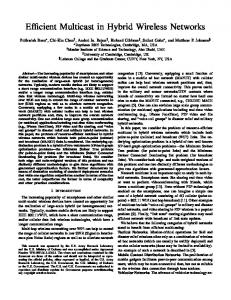
2 Figures 3 and 4 show the node degrees and diameters of various network topologies as a function of the network size. Degree at most equal to 5 seems to be sufficient for network sizes that are expected to be practical in the near future. Although the HCN [21], RCC [23], and HSN [51] topologies also have small node degree and diameter, and possess several desirable algorithmic properties, they are asymmetric and irregular, and their node degrees are in general larger than those of MS networks. CCC [41] and SCC [32] have degree equal to 3, but their diameter and algorithmic properties are not as good as those of MS networks. MS networks are also competitive in terms of the cost measure, defined as the diameter times node degree [13], as shown in Fig. 5. Even though the diameter of an interconnection network determines its delay under light load conditions, congestion becomes the limiting factor on the performance when the network load is large. It is therefore important that the utilization of the links is close to uniform, at least when the sources and destinations of the packets are uniformly distributed over all network nodes. The following theorem shows that this is indeed the case for the MS(l ; n) network when l = Θ(n). 14

Corollary 3.3 When the sources and destinations of the packets are uniformly distributed over all nodes of an MS(l ; n) network with l = Θ(n), and the routing algorithms described in Subsections 2.1, 3.1, and 3.2 are used, the expected traffic on the network links is equally balanced within a constant factor. Proof (abbreviated): This can be shown by computing the probability with which each link is used. The expected traffic on all inter-cluster links (also, on all nucleus links) in an MS network is the same due to symmetry. The expected traffic on an inter-cluster link is inversely proportional to l ? 1, while the expected traffic on a nucleus link is inversely proportional to n. Thus, the expected traffic is equally balanced within a constant factor on all network

2

links when l = Θ(n). The number l of hierarchical levels in an N-node MS(l ; n) network is given by l=Θ



log N n log log N

 (2)

:

Equation (1) together with Eq. (2) imply that the node degree d = n + l ? 1 of an MS(l ; n) network is minimized when l = Θ(n) = Θ

q

log N log log N



, leading to the following lemma.

Lemma 3.4 The node degree of an N-node MS(l ; n) network is minimized and is equal to Θ

q

log N log log N

 if and only

if l = Θ(n). Since n + l ? 1  nl

=

 O

log N log log N



for any positive integers n and l, the node degree of an N-node MS(l ; n)

network can take values in the range from Ω

q

log N log log N



to O



log N log log N



, depending on the particular choice of the

parameters n and l. As we will see later, the condition l = Θ(n), which leads to balanced traffic on all network links (Corollary 3.3) and guarantees minimal node degree (Lemma 3.4), also results in the best diameter to lower-bound ratio (Subsection 3.4), and optimal emulation of the star graph under both the single dimension and the all-port communication models (Subsection 4.2). Moreover, the expected traffic is also uniform for algorithms emulating the star graph, assuming uniformly generated packets for neighboring nodes (Section 4). As a consequence, all these desirable properties can be achieved at the same time on an MS(l ; n) network with l = Θ(n). In what follows, we will informally refer to an MS(l ; n) network with l = Θ(n) as a balanced MS network.

3.4 Near Optimal Diameter Let G be an undirected interconnection network that has N nodes, degree d  3, and diameter D(G). We then have N  1+d

d (d ? 1)D G ? 2 i?1 ? 1 ) = (Moore’s bound) ∑ d?2

D(G)

( )

(d

i=1

15


logd?1 N + logd?1 (1 ? 2=d )

(3)

4

on the diameter D(G). Note that the lower order term c(d ) = logd?1 (1 ? 2=d ) satisfies c(d )  ? log2 3 for any d  3

and approaches 0 very fast when d increases (for example, c(4)  ?0:631 and c(7)  ?0:19). We define the universal

lower bound DL (N ; d ) on the diameter of a static undirected interconnection network that has N nodes and degree d  3 as

DL (N ; d ) = logd?1 N + logd?1 (1 ? def

2 ): d

(4)

For a given graph G, we define the asymptotic diameter to lower-bound ratio D(G) : N!∞ DL (N ; d )

a(G) = lim

Note that a(G)  1, and small values of a(G) are desirable. A graph G will be said to have (asymptotically) optimal diameter if the ratio a(G) is a constant, or equivalently, if the diameter of G is asymptotically within a constant factor from the lower bound. Theorem 3.5 Any MS network has asymptotically optimal diameter. Proof: By substituting the node degree d < k = O



log N log log N





(Eq. (1)) into Eq. (4), we get

log N DL (N ; d ) = Ω log log N

 ;

which is of the same order of magnitude with the diameter of any N-node MS network (Theorem 3.2).

16

2

Corollary 3.6 The asymptotic diameter to lower-bound ratio of the MS(l ; n) network is a(MS(l ; n)) = 1:25, when l = Θ(n) [that is, when the MS network is balanced]. Proof: Using Equation (4) together with Stirling’s approximation [22], we have DL (N ; d ) =

log2 k! k log2 k ? O(k) o(1) = ? : log2 (n + l ? 2) log2 (n + l ? 2)

For l = Θ(n), we have log2 l = log2 n  O(1), and the universal lower bound on the diameter becomes D L (N ; d ) =

k(2 log2 n  O(1)) log2 n + O(1)



k = 2k  O log n



:

By Theorem 3.2, the diameter of the MS(l ; n) network is equal to 2:5k + O(l ), which gives an asymptotic diameter to lower-bound ratio of a(MS(l ; n)) = 2:5=2 = 1:25;

2

when l = Θ(n). For l = Θ(n), the N-node MS(l ; n) network has node degree

s d=Θ and diameter

p

2:5k + O( k) =

log N log log N

!



2:5 log2 N log N +o log2 log2 N log log N



(from Eq. (1)), both of which are sub-logarithmic. The asymptotic diameter to lower-bound ratios for the balanced MS network and several other interconnection networks of interest are summarized in Table 1. Although diameter and average distance may be less important for networks using wormhole routing under light traffic, they are crucial for network performance under heavy load. The maximum throughput of a network is inversely proportional to these parameters for any switching technology. In [17, 2], it has been shown that lowerdimensional k-ary n-cubes perform better than higher-dimensional ones under the constraint of constant bisection bandwidth. In [1], Abraham and Padmanabhan examined network performance under pin-out constraints and showed that higher-dimensional networks performed better. Generally speaking, low-dimensional k-ary n-cubes outperform MS networks under the bisection-bandwidth constraint; while MS networks outperform k-ary n-cubes and hypercubes under constant pin-out constraint. Detailed comparisons based on such considerations are outside the scope of this paper.

17

Table 1. Asymptotic diameter to lower-bound ratios of various interconnection networks with N nodes. Graph Hypercube

Degree log2 N 

log2 N log2 log2 N + o

Star Graph d-dimensional mesh de Bruijn Graph‡ CCC

2d 4 3

SCC

3

balanced MS(l ; n) †

‡

q 2

log2 N log2 log2 N + o

log N log log N

Diameter log2  N



1:5log2 N log2 log2 N + o

log N log log N



1:5

Θ(N 1 d ) log2 N 2:5 log2N ? O(loglog N ) =

q

log N log log N



Θ

log2 N



(log log N)2

2:5log2 N log2 log2 N + o

log N log log N

a(G)† log2 log2 N



1=d

d Θ( N loglog N ) 1:73  2:5 

Θ

log N

(log log N)2

1:25

When N is not large, the actual diameter to lower-bound ratio D(G)=DL (N; d ) is larger than the asymptotic ratio a(G) indicated in the table for star graphs and MS networks, and smaller than that for CCC networks. The binary de Bruijn graph is viewed as an undirected degree-4 network.

4 Parallel Algorithms in MS networks In this section, we show how to emulate algorithms developed for a k-dimensional star graph on an MS(l ; n) network. In our emulation algorithms, a node in the k-star is one-to-one mapped on the node that has the same permutation label in the MS(l ; n) network.

4.1 Parallel Algorithms under the Single-Dimension Communication Model In this subsection, we assume the single-dimension communication (SDC) model, where the nodes are allowed to use only links of the same dimension at any given time. This communication model is used in some SIMD architectures to reduce the cost of implementation, and is also suitable for parallel systems that use wormhole routing. Many algorithms developed for the star graph fall into this category [38]. Two basic communication tasks that arise often in applications are the multinode broadcast (MNB) and the total exchange (TE) [12, 27, 48, 49]. In the MNB each node has to broadcast a packet to all the other nodes of the network, while in the TE each node has to send a different (personalized) packet to every other node of the network. Miˇsi´c and Jovanovi´c [38], have proposed strictly optimal algorithms to execute both tasks in time k! ? 1 and (k + 1)! + o((k + 1)!)‡ , respectively, in a k-star with single-dimension communication. Using Theorem 3.1, the algorithms proposed in [38] give rise to corresponding asymptotically optimal algorithms for the MS(l ; n) network. Corollary 4.1 The total exchange task can be performed in time Θ ‡ The

notation f (N) = o(g(N)) means that limN!∞ f (N)=g(N) = 0:

18



N log N log log N

 in an N-node MS network under the

SDC model. This completion time is asymptotically optimal for the total exchange task over all interconnection networks that have N nodes and degree O(logc N ), where c = O(1), assuming single-port communication. Proof: The completion time follows from Theorem 3.1 through emulating the TE algorithm given in [38]. The lower bound can be proved by arguing that any interconnection network with N nodes of degree O(logc N ) has mean internodal distance of at least Ω



log N log log N



. (The derivation is similar to that given in Subsection 3.4 for the lower bound

on the diameter.) Therefore, the total number of packet transmissions required to execute the TE task is Ω



N2 log N log log N



.

Since at most N transmissions (one per node) can take place simultaneously under the single-port communication

2

model, the corollary follows.

When the dimensions of the links used by an algorithm in the star graph are consecutive, the algorithm can be emulated even more efficiently, often with a slowdown factor of 1 asymptotically. We present this result formally in the following theorem. Theorem 4.2 Any algorithm in a k-star using links of consecutive dimensions j; j + 1; :::; j + s ? 1 in s consecutive

steps can be emulated on the MS(l ; n) network in time s ? 2a1 + 2b1 + 2c1 ; where a1 = b( j ? 2)=nc, b1 = b( j + s ? 2)=nc, and

 c1 =

1 0

if a1 > 0; otherwise.

Proof: If we emulate the transmissions over two successive dimensions j + t and j + t + 1 using the algorithm given in Theorem 3.1, each node U has to route packets via links (from left to right) St1 +1 ; Tt0 +2 ; St1 +1 ; St1 +1 ; Tt0 +3 ; St1 +1 ; where t0 = ( j + t ? 2) mod n and t1 = b( j + t ? 2)=nc, assuming t0 6= n ? 1. Clearly, the third and fourth routing steps cancel each other and can be removed, and the emulation requires transmissions over links St1 +1 ; Tt0 +2 ; Tt0 +3 ; St1 +1 : Note that each node St1 +1 (U ), which receives data from node U in the first step, has to emulate the required computation on node U. When t0 = n ? 1, different inter-cluster links will be used in the third and fourth routing steps above, for a total of

exactly 2b1 ? 2a1 steps that cannot be eliminated by the above method. Two steps (routing on Sa1 links) are required

at the beginning and end of the emulation algorithm when a1 6= 0. Thus, 2b1 ? 2a1 + 2c1 extra steps are required to

emulate the s steps of the algorithm on the (nl + 1)-star, which completes the proof.

2

Using Theorem 4.2, we can emulate a number of star graph algorithms on an MS network with a slowdown factor smaller than 3. In particular, we can obtain an asymptotically optimal algorithm (within a factor of 1) to execute the 19

multinode broadcast task in an MS network, by emulating the corresponding algorithm given in [38] for star graphs, leading to the following corollary. Corollary 4.3 The multinode broadcast task can be performed in time N + o(N ) in an N-node MS network under the SDC model.

4.2 Emulation of Star Graphs under the All-Port Communication Model We now consider the all-port communication model, where a node is allowed to use all its incident links for packet transmission and reception at the same time. The packets transmitted on different outgoing links of a node can be different. Given two graphs G1 and G2 of similar sizes, and node degrees d1 and d2 , a lower bound on the time required for G1 to emulate G2 is T (d1 ; d2 ) = dd2 =d1 e. When G1 can emulate G2 with a slowdown of Θ(T (d1 ; d2 )), we will say that graph G1 can (asymptotically) optimally emulate graph G2 . In what follows, we show that an MS(l ; n) network can emulate a star graph of the same size with asymptotically optimal slowdown. Theorem 4.4 Any algorithm in a k-star with all-port communication can be emulated on the MS(l ; n) network with a slowdown factor of max(2n; l + 1). Proof: In Theorem 3.1, we have shown that an MS(l ; n) network can emulate an (nl + 1)-star with a slowdown factor of 3 under the SDC model. The emulation algorithm with all-port communication simply performs single-dimension emulation for all dimensions at the same time with proper scheduling to minimize the congestion. In particular, a packet for a dimension- j neighbor, j  n + 2, in the emulated star graph will be sent through links S j1 +1 ; T j0 +2 ; S j1 +1 , where j0

=

j ? 2 mod n and j1

b ? 2) nc.

= (j

=

There exist several schedules that guarantee the desired slowdown

factor. In what follows we present such a possible schedule. We first consider the special case where l = rn + 1 for some positive integer r.



At time 1, each node sends the packets for its dimension- j neighbors (in the emulated k-star), j = 2; 3; 4; : : : ; n + 1, through links T j .



At time t, t



At time t, t

=

1; 2; 3; : : : ; n, each node sends the packets for its dimension-ui (t ) neighbors, i

=

2; 3; 4; : : : ; l,

through links Si , where ui (t ) = (i ? 1)n + 2 + (i + t ? 3 mod n). =

sn + 2; sn + 3; sn + 4; : : : ; (s + 1)n + 1 for s = 0; 1; 2; : : : ; r ? 1, each node forwards the packets

for dimension-vi (t ) neighbors, i = sn + 2; sn + 3; sn + 4; : : : ; (s + 1)n + 1, through links Tvi (t ) , where vi (t ) = (i



? 1)n + 2 + (i + t ? 2sn ? 4 mod n).

At time t, t = n + 1; n + 2; : : : ; 2n, each node forwards the packets for its dimension-ui (t ) neighbors, i = 2; 3; 4; : : : ; n + 1, through links Si , where ui (t ) = (i ? 1)n + 2 + (i + t ? n ? 3 mod n). 20

JHQHUDWRUV RIDQ06 QHWZRUN

6WHS



6WHS



6WHS



6WHS



6WHS



6WHS



GLPHQVLRQRIWKHVWDUEHLQJHPXODWHG M  7 7 7 6







6





7 6



7 6

6



6 

7

7



 

7 6



6







7 7 6







6 

6



6



6



6 

6 

GLPHQVLRQRIWKHVWDUEHLQJHPXODWHG M

7 7 7 6





6

6 

6WHS



7 

6WHS



7 6

6WHS



7

6WHS



6WHS



6WHS



6 

7 



JHQHUDWRUV

RIDQ06 QHWZRUN 

6 









6



6 

6

7

7

7

6 





6



6 







6



D

7



6



6



7



6





6 

6

7 

7

6 

7 





6



6



6 7



6 

7 

6 

6 



6



6



E

Figure 6: Schedules for emulating star graphs on MS networks, under the all-port communication model. Note that a generator appears at most once in a row, and each column j > 4 consists of generators S j1 +1 ; T j0 +2 ; S j1 +1 , where j0 = j ? 2 mod 3 and j1 = b( j ? 2)=3c. (a) Emulating a 13-star on an MS(4; 3) network. (b) Emulating a 16-star on an MS(5; 3) network. The links in the MS network are fully used during steps 1 to 5, and are 93% used on the average.



At time t, t

=

sn + 3; sn + 4; sn + 5; : : : ; (s + 1)n + 2 for s = 1; 2; 3; : : : ; r ? 1, each node forwards the packets

for dimension-ui (t ) neighbors, i = sn + 2; sn + 3; sn + 4; : : : ; (s + 1)n + 1, through links Si , where ui (t ) = (i ?

1)n + 2 + (i + t ? 2sn ? 5 mod n).

Figure 6a shows such a schedule for emulating a 13-star on an MS(4; 3) network. In what follows we extend the previous schedule to the general case where l is not of the form l

=

rn + 1. The

schedule for l  n can be easily obtained by removing the unused part of the schedule for an MS(n + 1; n) network.

Other possible cases can be formulated by assuming that l = rn ? w for some integers r  2 and 0  w  n ? 2, in which case we can modify the schedule as follows. We initially start with the schedule for an MS(rn + 1; n) network. Clearly, the transmissions in the schedule that correspond to the emulation of dimensions j > ln + 1 are not used by the MS(l ; n) network. Therefore, we can now perform each of the transmissions over links T j0 +2 originally scheduled for time l + 1 through rn + 1 at time earlier than l + 1 by rescheduling these transmissions to the unused part of the schedule. Note that the modified part of the schedule are for the emulation of some dimensions larger than (r ? 1)n2 + n + 1 (that is, some of the dimensions that correspond to the last l ? (r ? 1)n ? 1 = n ? w ? 1 blocks). We then swap

generators T j0 +2 in the modified part of the schedule with part of the schedule for the emulation of dimensions smaller

than (r ? 1)n2 + n + 2 (that is, for some of the dimensions that correspond to the first (r ? 1)n + 1 blocks). Due to the

previous modifications, we also have to move the schedule for some generators S j1 +1 . In particular, we will move the final generator S j1 +1 in each of the 3-step single-dimension emulations one time step after the use of T j0 +2 generators when possible. When l + 1 < 2n, the schedule for some generators S j1 +1 can not be moved before time 2n. As a result, the time required for emulation under the all-port communication model is equal to l + 1 if l + 1  2n, and is equal to 2n otherwise. Figure 6b shows such a schedule for emulating a 16-star on an MS(5; 3) network.

21

2

By properly choosing the parameters l and n, we can emulate a star graph with all-port communication on an MS(l ; n) network with asymptotically optimal slowdown with respect to the node degrees. Corollary 4.5 Any algorithm in a k-star with all-port communication can be emulated on the MS(l ; n) network with

h

asymptotically optimal slowdown if l = Θ(n) or equivalently, if the node degree is Θ Proof: It follows from Lemma 3.4, Theorem 4.4, and the fact that a graph of degree Θ graph of degree Θ

2



log N log log N



with a slowdown smaller than Θ

Note that the slowdown factor of Θ

q

log N log log N



q

log N log log N

q

q



log N log log N

log N log log N

i

.

 cannot emulate a

, under the all-port communication model.

is also the congestion for embedding a k-star on an MS(l ; n) net-

work with l = Θ(n). Therefore, no graph that has N nodes and degree Θ

q

log N log log N



can embed an N-node star graph

with asymptotically better congestion (by more than a constant factor) than that achieved by an MS(l ; n) network with l = Θ(n). Fragopoulou and Akl [20] have given optimal algorithms to execute the multinode broadcast (MNB) and the total exchange (TE) communication tasks in a k-star with all-port communication in time Θ((k ? 1)!) = Θ(N log log N = log N ) and Θ(k!) = Θ(N ), respectively. Emulating their algorithms leads to the following asymptotically optimal algorithms for MS networks.

 q

Corollary 4.6 The multinode broadcast task can be performed in time Θ N

log log N log N



in an MS(l ; n) network with

l = Θ(n). This completion time is asymptotically optimal for the multinode broadcast task over all interconnection networks that have N nodes and degree Θ

q

log N log log N



, under the all-port communication model.

 q

Corollary 4.7 The total exchange task can be performed in time Θ N

log N log log N



in an MS(l ; n) network with l

=

Θ(n). This completion time is asymptotically optimal for the total exchange task over all interconnection networks that have N nodes and degree Θ

q

log N log log N



, under the all-port communication model.

Proof: Since the TE can be performed in an N-node star graph in time Θ(N ) [20], it can be completed in time

 q

O N

log N log log N



in an MS(l ; n) network with N nodes of degree Θ

assuming all-port communication and l

=

q

log N log log N



through emulation (Theorem 4.4),

Θ(n). By arguing as in the derivation of the universal diameter lower

bound DL (d ; N ), we can show that the mean internodal distance of an N-node graph with degree Θ least Ω Ω





log N log log N

N2 log N log log N





q

log N log log N



is at

. The total number of packets that have to be exchanged to perform a TE is N 2 ? N, for a total of

 q

packet transmissions. Since at most O N

N-node interconnection network of degree Θ

q

log N log log N



log N log log N



transmissions can take place simultaneously in an

under the all-port communication model, the time required

22

to complete the TE is at least Ω

N

N 2 logN log logN log N loglogN

q

! =Ω

 q N

log N log log N

 :

2

4.3 Embeddings of Trees, Meshes, Hyprcubes, and Complete Transposition Graphs In this subsection, we present constant-dilation embeddings of several important graphs in MS networks. The following corollary follows directly from Theorem 3.1. Corollary 4.8 A k-star graph can be one-to-one embedded in an MS(l ; n) network with load 1, expansion 1, and dilation 3. A k-dimensional complete transposition graph CT(k) [34, 35] is a Cayley graph defined with a generator set consisting of all the generators that interchange any two of the k symbols in the label of a node. A CT(k) graph has k! nodes, degree k(k ? 1)=2, and diameter k ? 1. It contains a k-star or a k-dimensional bubble-sort network [5] as a subgraph and has been shown to be a rich topology that can efficiently embed many other popular topologies, including hypercubes, meshes, and trees. The following theorem provides O(1)-dilation embedding of complete transposition graphs in macro-star networks. Theorem 4.9 A k-dimensional complete transposition graph can be one-to-one embedded in an MS(l ; n) network with load 1, expansion 1, and dilation 5 when l = 2, or dilation 7 when l  3. Proof: Similar to Theorem 3.1, we map each node in the CT(k) graph onto the node with the same label in the MS(l ; n) network. Therefore, the load and expansion of the embedding are both equal to 1. We let Ti j be the generator that ;

interchanges the

ith

and

jth

symbols in the label of a node, where 1  i < j. Then the generator set for a CT (k) graph

consists of generators Ti j for any combination of integers i; j satisfying 1  i < j ;

 k.

Letting i0

=

i1 = b(i ? 2)=nc, j0 = j ? 2 mod n, and j1 = b( j ? 2)=nc, it is easy to verify the following equivalence

8 Tj > > > > TS S > > < T jT1 +T1 j i1 +1 i j i Ti j = T > i > S j1 +1 T j0 +2 S j1 +1 Ti > > > T T T S > : Si1 +1 i0 +2 j0 +2 i0 +2 i1 +1 ;

Si1 +1 Ti0 +2 S j1 +1T j0 +2 S j1 +1 Ti0 +2 Si1 +1

i ? 2 mod n,

8 i = 1; j1 = 0; > > > > i = 1; j1 > 0; > > > i1 = 0; j1 > 0; > > > > : i1 = j1 > 0;

i1 6= j1 ; i1 ; j1 > 0:

As a result, the dilation for embedding a CT(k) graph in an MS(l ; n) network is at most equal to 7. When l = 2, only the first five cases are possible, so that the dilation is equal to 5 for an MS(2; n) network.

23

2

Since a k-dimensional bubble-sort network is a subgraph of a CT (k) graph, it can also be embedded it in an MS(l ; n) network with dilation 5 when l = 2, and dilation 7 when l  3. A variety of embedding results are available for star graphs, bubble-sort graphs, and complete transposition graphs [14, 34, 37, 28]. These results, when combined with Theorem 4.9 and Corollary 4.8, give rise to a variety of O(1)dilation embeddings for MS networks. The following corollaries summarize some of the results. Corollary 4.10 There exists a dilation-3 embedding of the complete binary tree of height 5 into an MS(2; 2) network. For k  7, there exists a dilation-3 embedding of the complete binary tree of height at least equal to (1=2 + o(1))k log2 k into an MS(l ; n) network. Proof: In [14], it has been shown that for k = 5 or 6 there exists a dilation-1 embedding of the complete binary tree of height 2k ? 5 into the k-star. For k  7, there exists a dilation-1 embedding of the complete binary tree of height at least equal to (1=2 + o(1))k log2 k into the k-star. The rest of the proof follows from Corollary 4.8.

2

Corollary 4.11 There exists a dilation-O(1) embedding of d-dimensional hypercube into an MS(l ; n), provided d  k log2 k ? 3k 2 + o(k).

Proof: In [37], it has been shown that there exists a dilation-O(1) embedding of the d-dimensional hypercube into a k-star, provided that d  k log2 k ? (3=2 + o(1))k. This, combined with Corollary 4.8, completes the proof.

2

Corollary 4.12 There exists a load-1, expansion-1, and dilation-5 embedding of the M1  M2 mesh into an MS(2; n)

network, where M1  M2 = (2n + 1)!. There exists a dilation-7 and expansion-1 embedding of the M1  M2 mesh into

an MS(l ; n) network, where M1  M2 = k! and l  3.

Proof: It follows from Theorem 4.9 and the fact that there exists a dilation-1 expansion-1 embedding of M1  M2 mesh into a CT(k) graph, where M1  M2 = k! [34].

2

Corollary 4.13 There exists a dilation-O(1) expansion-1 embedding of the 2  3  4 


 (k ? 1)  k mesh into an MS(l ; n) network. Proof: In [28] it has been shown that there exists a dilation-3 expansion-1 embedding of the 2  3  4 


 (k ? 1)  k mesh into a k-star. This, combined with Corollary 4.8, completes the proof.

2

5 Implementation Considerations In previous sections, we have shown various theoretical advantages of MS networks. In this section, we address some practical and implementation issues, and provide a detailed comparison between MS networks and star graphs. 24

5.1 Scaling up MS Networks An MS(l ; n) network has N = (nl + 1)! nodes and degree equal to n + l ? 1. For a given N = k!, there may be more than one MS(l ; n) network with N processors, because there may be more than one pair (l ; n) for which k = nl + 1. Two networks MS(l1 ; n2 ) and MS(l2 ; n2 ) that have the same number of nodes (i.e., l1 n1 = l2 n2 ) may have different degrees l1 + n1 ? 1 and l2 + n2 ? 1 and different diameters. For a given number of nodes N = k! = (nl + 1)!, it is generally preferable to have l = Θ(n) so that the network is balanced (see Sections 3 and 4). Clearly, this is not always possible (e.g., if k ? 1 is prime), which implies that when

scaling up an MS(l ; n) network with k! = (ln + 1)! nodes to obtain an MS(l 0 ; n0 ) network with (k + 1)! = (l 0 n0 + 1)! nodes, many of the original properties may not be preserved. For example, consider scaling up an MS(3; 4) network that has 13! nodes to the (only) MS(13; 1) network that has 14! nodes (the immediately next possible number of nodes). The MS(3; 4) network is close to being balanced and has degree equal to 6, while the MS(13; 1) network has degree equal to 13. Furthermore, the MS (13; 1) network does not contain the MS(3; 4) network as a subgraph. If modularity in the design is to be preserved, the MS network should be scaled up by increasing the number of levels l by one, keeping parameter n constant. To obtain an MS(l + 1; n) network from an MS(l ; n) network, n additional symbols have to be used in the node label, increasing the number of nodes by a factor of

(nl +n+1)! (nl +1)!

. Such a step size may be too large for practical applica-

tions. This problem is common to other hierarchical modular networks, such as hypernets [25], RCC [23], and HSN [51]. In what follows, we briefly present alternative ways to scale up an MS network with a smaller step size, while preserving most of its desirable properties, and ensuring modularity in the design. The first method is to allow more flexible connectivity at the top level. For example, consider a network that consists of (k + m)!=k!, 1  m  n, identical copies of an MS(l ; n) network. A node in this variant network is repre-

sented by k + m symbols, where 1  m  n, and is connected through an additional link to a new neighbor, obtained

by swapping the first m symbols with the last (additional) m symbols of the node label. We call this an incomplete MS network and we denote it by IMS((m); l + 1; n). For example, the IMS((1); 3; 3) network has 8! nodes and generators def

def

T2 ; T3 ; T4 ; S3 2 (I) = 1 567 234 8; and S(1) 3 3 (I) = 1 8 34 567 2: ;

; ;

IMS((m); l + 1; n) networks have properties similar to those of MS (l + 1; n) networks, and most of the results derived in this paper can be applied to them either directly (for example, the emulation algorithms presented in Section 4) or after minor modifications (for example, the routing algorithms). In particular, to extend the MS routing algorithm introduced in Section 3 to IMS networks, we have to perform a complete SDC emulation (involving 3 steps) when an exchange with a symbol within the rightmost block is involved, while the rest of the algorithm remains the same. An upper bound on the diameter of IMS((m); l ; n) networks can be shown to be 2:5nl + O(n + l ). The tech25

nique used above can be further generalized to provide more flexibility at lower levels. For example, we can use generators T2 ; T3 ; T4 , S(2) 3 2 (I) = 1 56 4 23 78; and S(2) 3 3 (I) = 1 78 4 56 23; to obtain an incomplete MS network, ; ;

; ;

IMS((2; 2); 3; 3), that has 8! nodes and degree 5. The integer numbers in the inner parenthesis indicate that the incomplete blocks 2 and 3 consist of 2 symbols each, rather than 3 symbols. It can also be seen that a Cayley graph [5] using generators T2 ; T3 ; T4 ; S(1) 3 2 (I) = 1 567 234 8; and S03 (I) = 1 678 5 234; as well as other variant topologies, ; ;

also have algorithms and properties similar to those of MS networks. Since the variants introduced so far belong to the class of Cayley graphs, they are all vertex-symmetric and regular. Similar to Theorem 3.1, it can be easily shown that all of them can embed a star graph of the same size with dilation 3. Similar to Theorem 4.9, it can be shown that all the variants introduced so far can embed a complete transposition graph of the same size with dilation 5 when the number of hierarchy levels is equal to 2, and with dilation 7 otherwise. As a result, the parallel algorithms presented in Subsections 4.1 and 4.3 can be directly applied to all these variants. Also , the results of Subsection 4.2 can be extended to them by performing SDC emulations for all dimensions with proper scheduling. A second method for scaling up an MS network with an even smaller step size uses a strategy similar to that used in the construction of the clustered star and incomplete star [33]. More precisely, some of the level-l clusters and the

n

o

corresponding links are removed from the MS (l ; n) network, leaving a total of c 2 2; 3; :::; (nl(nl?+n+1)1!)! level-l clusters that are not removed. We call the resultant topology a clustered MS network, and we denote it by CMS((c); l ; n). Clearly, all the algorithms presented in this paper can be applied to each of the c level-l clusters in the CMS((c); l ; n) network. The number of nodes in a CMS network can be increased by a factor of 1 + 1c by adding an additional level-l cluster. This construction can be further generalized by allowing clusters at lower levels to be removed. Also, the techniques used in the construction of the IMS and the CMS networks can also be combined to obtain even more flexible variant topologies. More precisely, an MS(l ; n) network can first be scaled up to obtain an IMS((m); l + 1; n)

n

+m+1)! network, and then some of its top-level clusters can be removed, leaving a total of c 2 2; 3; :::; (nl(nl +1)!

o

top-level

clusters that are not removed. In general, the variants obtained by the second method are not Cayley graphs, and they are not symmetric or regular. Techniques similar to those used in the derivation of Cayley coset graphs [24] can also be used to obtain other variant topologies that have a small step size.

5.2 Mapping of MS Networks onto Parallel Architectures With the rapid advances in VLSI technologies, the number of transistors and the number of processors that can be put onto a chip are expected to grow significantly. Since the processor-memory bandwidth is one of the major bottlenecks limiting the performance of current and future parallel systems, implementing processors in memory (PIM) [30, 15] or computing in RAM [46, 47] offer a lot of promise for the construction of future parallel computers. Another trend

26

in the synthesis of multicomputers is to use off-the-shelf PC or workstation boards (or processor chips) as building modules. In either case, the number of available off-module (e.g., off-chip or off-board) pins is one of the major constraints limiting the number of processors that can be put on the module. Also, the inter-module bandwidth is a potential bottleneck on the performance of the resultant system. In what follows, we consider the case where several nodes (processors, routers, and their memory banks) of an MS network are implemented on a single chip, or more generally, a single module. EXECUBE [30, 47], hypernets [25, 26], WK-recursive networks [18], and hierarchical shuffle-exchange networks (HSE) [16] are some of the well-known parallel architectures and networks that use such an approach or similar assumptions. A natural partition of the processors (and their memory banks and network interfaces) of an MS(l ; n) network into chips is to put all processors belonging to the same nucleus (n + 1)-star onto the same chip. The MS(l ; n) network can then be built with identical chips, which are connected to other chips through swap links. This partition also eliminates the “number of parts” problem since it uses identical building modules. We expect that 3-star and 4-star (or at most 5-star) modules will be sufficient to build MS-based multicomputers for most practical purposes (see Table 2). For example, an MS network with 7!  5K nodes can be implemented as an MS(3; 2) built from identical 3-star chips, with each node in the chip requiring 2 off-chip links, or an MS(2; 3) network built from identical 4-star chips, with each node in the chip requiring only 1 off-chip link. For comparison, a 7-star built with 3-star or 4-star chips requires 4 or 3 off-chip links per node, respectively. Since many well known topologies use rings as their basic building modules (e.g., the CCC, SCC, ring of rings, hierarchical ring, and Cayley-graph-connected cycles [39]), or contain rings as subgraphs (e.g., meshes, hypercubes, and tori), it is quite possible that off-the-shelf ring modules (having a limited number of off-module links) will be commercially available in the future. This would make MS networks built from such modules considerably less expensive than parallel computers built from customer-designed modules. Since star graphs are viewed as attractive candidates for future parallel computers, it is also possible that modules used to build small or medium-scale star-graph will be available and could be used to build larger-scale MS networks. For example, multicomputers based on the 6-star or larger star graphs may be built from 4-star modules, with each node having at least 2 off-module links; these 4-star modules can also be used to build MS(3; 3) network with 10!-node or IMS networks with 7!, 8!, or 9! nodes. Moreover, the 7!, 8! or 9!-node IMS networks can later be expanded to larger networks using the same basic modules. For comparison, if we want to build a k-star with k = 8; 9, or 10, using 4-star chips, the required numbers of off-chip links per node will be 4, 5, or 6, respectively, resulting in larger hardware costs and may not be commercially available. In general, k-stars with k = 6; 7; 8; 9 can not be expanded to larger star graphs in the future using the same modules, because their node degrees increase with network size. Table 2 summarizes the above discussion by comparing several options for building parallel computers based

27

Table 2: Comparison of MS and IMS networks and star graphs in terms of the node degree and the number of off-module links per node. 1RGHV

1HWZRUN

'HJUHH

%DVLF0RGXOH

1XPEHURIRIIPRGXOH



VWDU



VWDU





VWDU



VWDU





VWDU



VWDU





VWDU



VWDU





06 06



VWDU





,06  ,06 



VWDU





,06  06



VWDU





06



VWDU



OLQNVSHUQRGH

on the MS, IMS, and star graph topologies in terms of implementation considerations, such as node degree, basic modules used, and number of off-module links per node.

6 Conclusions Desirable properties in interconnection networks for parallel systems include small network diameter, symmetry, modularity, ease of mapping efficient algorithms onto them, and reasonable implementation cost. The hypercube and star graph meet most of these requirements, but their node degrees are prohibitively large for networks of large size. The MS networks proposed in this paper form a new class of interconnection networks for the modular construction of parallel computers. MS networks have several desirable algorithmic and topological properties, while using nodes of small degree. We showed that MS networks have asymptotically optimal diameter, and we presented efficient algorithms to perform routing in them. We also developed efficient algorithms to emulate the star graph, and asymptotically optimal algorithms to execute the MNB and TE communication tasks, under both the single-port and the all-port communication models. In all routing algorithms presented, the expected traffic was shown to be balanced on all links of the MS(l ; n) network with l = Θ(n). We presented variants of the MS network that are more flexible to scale up, and can be more easily adjusted to the size of a particular application. We also compared MS networks and star graphs with respect to several practical implementation considerations. We believe that the MS network and its variant topologies can fit the needs of high-performance interconnection networks, and appear to be efficient low-degree alternatives to the star graph for building medium to large-scale parallel architectures.

References [1] Abraham, S. and K. Padmanabhan, “Performance of multicomputer networks under pin-out constraints,” J. Parallel Distrib. Comput., Vol. 12, no. 3, Jul. 1991, pp. 237-248. [2] Agarwal, A., “Limits on interconnection network performance,” IEEE Trans. Parallel Distrib. Sys., Vol. 2, no. 4, Oct. 1991, pp. 398-412.

28

[3] Akers, S.B., D. Harel, and B. Krishnamurthy, “The star graph: an attractive alternative to the n-cube,” Proc. Int’l Conf. Parallel Processing, 1987, pp. 393-400. [4] Akers, S.B. and B. Krishnamurthy, “The fault tolerance of star graphs,” Proc. Int’l Conf. Supercomputing, Vol. III, 1987, pp. 270-276. [5] Akers, S.B. and B. Krishnamurthy, “A group-theoretic model for symmetric interconnection networks,” IEEE Trans. Comput., Vol. 38, Apr. 1989, pp. 555-565. [6] Akl, S.G., K. Qiu, and I. Stojmenovic, “Fundamental algorithms for the star and pancake interconnection networks with applications to computational geometry,” Networks, Vol. 23, Jul. 1993, pp. 215-225. [7] Akl, S.G. and K.A. Lyons, Parallel Computational Geometry, Prentice Hall, Englewood Cliffs, NJ, 1993. [8] Azevedo, M.M., “Star-based interconnection networks and fault-tolerant clock synchronization for large multicomputers,” Ph.D. dissertation, Dept. Electrical & Comp. Eng., Univ. of California, Irvine, 1997. [9] Bagherzadeh, N., M. Dowd, and S. Latifi, “Faster column operations in star graphs,” Dept. Elec. & Comput. Engr., Univ. California, Irvine, CA, Tech. Rep. ECE-94-02-01. [10] Bagherzadeh, N., M. Dowd, and S. Latifi, “A well-behaved enumeration of star graphs,” IEEE Trans. Parallel Distrib. Sys., Vol. 6, no. 5, May 1995, pp. 531-535. [11] Basak D. and D.K. Panda, “Designing clustered multiprocessor systems under packaging and technological advancements,” IEEE Trans. Parallel Distrib. Sys., Vol. 7, no. 9, Sep. 1996, pp. 962-978. [12] Bertsekas, D.P. and J. Tsitsiklis, Parallel and Distributed Computation – Numerical Methods, Prentice Hall, New Jersey, 1989. [13] Bhuyan, L.N. and D.P. Agrawal, “Generalized hypercube and hyperbus structures for a computer network,” IEEE Trans. Comput., Vol. 33, no. 4, Apr. 1984, pp. 323-333. [14] Bouabdallah, A., M.C. Heydemann, J. Opatrny, and D. Sotteau, “Embedding complete binary trees into star networks,” Proc. Int’l Symp. Mathematical Foundations of Computer Science, 1994, pp. 266-275. [15] Clark, D., Proc. NSF Workshop Critical Issues in Computer Architecture Research, May 1996. [16] Cypher, R. and J.L.C. Sanz, “Hierarchical shuffle-exchange and de Bruijn networks,” Proc. IEEE Symp. Parallel and Distributed Processing, 1992, pp. 491-496. [17] Dally, W.J. “Performance analysis of k-ary n-cube interconnection networks,” IEEE Trans. Comput., Vol. 39, no. 6, Jun. 1990, pp. 775-785. [18] Della Vecchia, G. and C. Sanges, “A recursively scalable network VLSI implementation,” Future Generations Comput. Sys., 1988, pp. 235-243. [19] Duh, D., G. Chen, and J. Fang, “Algorithms and properties of a new two-level network with folded hypercubes as basic modules,” IEEE Trans. Parallel Distrib. Sys., Vol. 6, no. 7, Jul. 1995, pp. 714-723. [20] Fragopoulou, P. and S.G. Akl, “Optimal communication algorithms on star graphs using spanning tree constructions,” J. Parallel Distrib. Computing., Vol. 24, 1995, pp. 55-71. [21] Ghose, K. and R. Desai, “Hierarchical cubic networks,” IEEE Trans. Parallel Distrib. Sys., Vol. 6, no. 4, Apr. 1995, pp. 427-435. [22] Graham, R.L., D.E. Knuth, and O. Patashnik, Concrete Mathematics: A Foundation For Computer Science, AddisonWesley, Menlo Park, CA, 1994. [23] Hamdi, M., “A class of recursive interconnection networks: architectural characteristics and hardware cost,” IEEE Trans. Circuits and Sys.–I: Fundamental Theory and Applications, vol. 41, no. 12, Dec. 1994, pp. 805-816. [24] Huang, J.-P., S. Lakshmivarahan, and S.K. Dhall, “Analysis of interconnection networks based on simple Cayley coset graphs,” Proc. IEEE Symp. Parallel and Distributed Processing, 1993, pp. 150-157. [25] Hwang, K. and J. Ghosh, “Hypernet: a communication-efficient architecture for constructing massively parallel computers,” IEEE Trans. Comput., Vol. 36, no. 12, Dec. 1987, pp. 1450-1466. [26] Hwang, K., Parallel Processing for Supercomputers and Artificial Intelligence, New York, McGraw-Hill, 1989.

29

[27] Johnsson, S.L. and C.-T. Ho, “Optimum broadcasting and personalized communication in hypercubes,” IEEE Trans. Comput., vol. 38, no. 9, Sep. 1989, pp. 1249-1268. [28] Jwo J.S., S. Lakshmivarahan, and S.K. Dhall, “Embedding of cycles and grids in star graphs,” Proc. IEEE Symp. Parallel and Distributed Processing, 1990, pp. 540-547. [29] Knuth, D.E., The Art of Computer Programming, Addison-Wesley, Reading, MA, 1973. [30] Kogge, P.M., “EXECUBE - a new architecture for scalable MPPs,” Proc. Int’l Conf. Parallel Processing, Vol. I, 1994, pp. 77-84. [31] Lakshmivarahan, S., J.-S. Jwo, and S.K. Dhall, “Symmetry in interconnection networks based on Cayley graphs of permutation groups: a survey,” Parallel Computing, Vol. 19, no. 4, Apr. 1993, pp. 361-407. [32] Latifi, S., M. Azevedo, and N. Bagherzadeh, “The star connected cycles: a fixed-degree network for parallel processing,” Proc. Int’l Conf. Parallel Processing, Vol. I, 1993, pp. 91-95. [33] Latifi, S. and N. Bagherzadeh, “Incomplete star: an incrementally scalable network based on the star graph,” IEEE Trans. Parallel Distrib. Sys., Vol. 5, no. 1, Jan. 1994, pp. 97-102. [34] Latifi, S. and P.K. Srimani, “Transposition networks as a class of fault-tolerant robust networks,” IEEE Trans. Parallel Distrib. Sys., Vol. 45, no. 2, Feb. 1996, pp. 230-238. [35] Leighton, F.T., Introduction to Parallel Algorithms and Architectures: Arrays, Trees, Hypercubes, Morgan-Kaufman, San Mateo, CA, 1992. [36] Menn, A. and Somani A.K., “An efficient sorting algorithm for the star graph interconnection networks,” Proc. Int’l Conf. Parallel Processing, Vol. III, 1990, pp. 1-8. [37] Miller, Z., D. Pritikin, and I.H. Sudborough, “Bounded dilation maps of hypercubes into Cayley graphs on the symmetric group,” Math. Sys. Theory, Vol. 29, no. 6, Springer-Verlag, Nov.-Dec., 1996, pp.551-572. [38] Miˇsi´c, J. and Z. Jovanovi´c, “Communication aspects of the star graph interconnection network,” IEEE Trans. Parallel Distrib. Sys., Vol. 5, no. 7, Jul. 1994, pp. 678-687. ¨ [39] Ohring, S., F. Sarkar, S.K. Das, and D.H. Hohndel, “Cayley graph connected cycles: a new class of fixed-degree interconnection networks,” Proc. Int’l Conf. Systems Sciences, 1995, pp. 479-487. [40] Parhami, B., Introduction to Parallel Processing: Algorithms and Architectures, Plenum Publishing Corp., 1998. [41] Preparata, F.P. and J.E. Vuillemin, “The cube-connected cycles: a versatile network for parallel computation,” Commun. of the ACM, Vol. 24, no. 5, May 1981, pp. 300-309. [42] Saikia, D.K. and R.K. Sen, “Order preserving communication on a star network,” Parallel Computing, Vol. 21, 1995, pp. 771-782. [43] Saikia, D.K. and R.K. Sen, “Two ranking schemes for efficient computation on the star interconnection networks,” IEEE Trans. Parallel Distrib. Sys., Vol. 4, Apr. 1996, pp. 321-327. [44] Scherson, I.D., and A.S. Youssef, Interconnection Networks for High-Performance Parallel Computers, IEEE Computer Society Press, 1994. [45] Sheu, J.-P., C.-T. Wu, and T.-S. Chen, “An optimal broadcasting Algorithm without message redundancy in star graphs,” IEEE Trans. Parallel Distrib. Sys., Vol. 6, no. 6, Jun. 1995, pp. 653-658. [46] Sterling, T., P. Messina, and P. Smith, Enabling Technologies for Peta(FL)OPS Computing, MIT press, 1994. [47] Sterling, T. and M.J. MacDonald, Proc. The PetaFLOPS Frontiers Workshop, 1995. [48] Varvarigos, E.A. and D.P. Bertsekas, “Communication algorithms for isotropic tasks in hypercubes and wraparound meshes,” Parallel Computing, Vol. 18, no. 11, Nov. 1992, pp. 1233-1257. [49] Varvarigos, E.A. and D.P. Bertsekas, “Multinode broadcast in hypercubes and rings with randomly distributed length of packets,” IEEE Trans. Parallel Distrib. Sys., Vol. 4, no. 2, Feb. 1993, pp. 144-154. [50] Yeh, C.-H. and E.A. Varvarigos, “Macro-star networks: efficient low-degree alternatives to star graphs for large-scale parallel architectures,” Proc. Symp. Frontiers of Massively Parallel Computation, Oct. 1996, pp. 290-297. [51] Yeh, C.-H. and B. Parhami, “Recursive hierarchical swapped networks: versatile interconnection architectures for highly parallel systems,” Proc. IEEE Symp. Parallel and Distributed Processing, Oct. 1996, pp. 453-460. [52] Yeh, C.-H. and B. Parhami, “Cyclic networks – a family of versatile fixed-degree interconnection architectures,” Proc. Int’l Parallel Processing Symp., Apr. 1997, 739-743.

30