Efficient Algorithms to Monitor Continuous Constrained k Nearest Neighbor Queries Mahady Hasan† , Muhammad Aamir Cheema† , Wenyu Qu‡ , Xuemin Lin† †
‡
The University of New South Wales, Australia {mahadyh,macheema,lxue}@cse.unsw.edu.au
College of Information Science and Technology, Dalian Maritime University, China
[email protected]
Abstract. Continuous monitoring of spatial queries has received significant research attention in the past few years. In this paper, we propose two efficient algorithms for the continuous monitoring of the constrained k nearest neighbor (kNN) queries. In contrast to the conventional k nearest neighbors (kNN) queries, a constrained kNN query considers only the objects that lie within a region specified by some user defined constraints (e.g., a polygon). Similar to the previous works, we also use grid-based data structure and propose two novel grid access methods. Our proposed algorithms are based on these access methods and guarantee that the number of cells that are accessed to compute the constrained kNNs is minimal. Extensive experiments demonstrate that our algorithms are several times faster than the previous algorithm and use considerably less memory.
1
Introduction
With the availability of inexpensive position locators and mobile devices, continuous monitoring of spatial queries has gained significant research attention. For this reason, several algorithms have been proposed to continuously monitor the k nearest neighbor (kNN) queries [1–3], range queries [13, 4] and reverse nearest neighbor queries [5, 6] etc. A k nearest neighbors (kNN) query retrieves k objects closest to the query. A continuous kNN query is to update the kNNs continuously in real-time when the underlying data issues updates. Continuous monitoring of kNN queries has many applications such as fleet management, geo-social networking (also called location-based networking), traffic monitoring, enhanced 911 services, locationbased games and strategic planning etc. Consider the example of a fleet management company. A driver might issue a kNN query to monitor their k closest vehicles and may contact them from time to time to seek or provide assistance. Consider another example of the location based reality game BotFighter in which the players are rewarded for shooting the other nearby players. To be able to earn more points, the players might issue a continuous kNN query to monitor their k closest players. We are often required to focus on the objects within some specific region. For example, a user might be interested in finding the k closest gas stations in NorthEast from his location. Constrained kNN queries [7] consider only the objects
that lie within a specified region (also called constrained region). We formally define the constrained kNN queries in Section 2.1. In this paper, we study the problem of continuous monitoring of constrained kNN queries. The applications of the continuous constrained kNN queries are similar to the applications of kNN queries. Consider the example of the fleet management company where a driver is heading towards the downtown area. The driver might only be interested in k closest vehicles that are within the downtown area. Consider the example of BotFighter game, the players might only be interested in the k closest players within their colleges so that they could eliminate their fellow students. Continuous constrained kNN queries are also used to continuously monitor reverse kNN queries. For example, six continuous constrained kNN queries are issued in [5, 8] to monitor the set of candidate objects. Similarly, constrained NNs are retrieved in [6] to prune the search space. Although previous algorithms can be extended to continuously monitor constrained kNN queries, they are not very efficient because no previous algorithm has been specifically designed for monitoring constrained kNN queries. In this paper, we design two simple and efficient algorithms for continuous monitoring of constrained kNN queries. Our algorithms significantly reduce the computation time as well as the memory usage. The algorithms are applicable to any arbitrary shape of constrained region as long as a function is provided that checks whether a point or a rectangle intersects the constrained region or not. Our contributions in this paper are as follows; – We introduce two novel grid access methods named Conceptual Grid-tree and ArcTrip. The proposed access methods can be used to return the grid cells that lie within any constrained region in order (ascending or descending) of their proximity to the query point. – We propose two efficient algorithms to continuously monitor constrained kNN queries based on the above mentioned grid access methods. It can be proved that both the algorithms visit minimum number of cells to monitor the constrained kNN queries. Our algorithms significantly reduce the computational time and the memory consumption. – Our extensive experiments demonstrate significant improvement over previous algorithms in terms of computation time and memory usage.
2 2.1
Background Information Preliminaries
Definition 1. Let O be a set of objects, q be a query point and R be a constrained region. Let OR ⊆ O be a set of objects that lie within the constrained region R, a constrained kNN query returns an answer set A ⊆ OR that contains k objects such that for any o ∈ A and any o′ ∈ (OR − A), dist(o, q) ≤ dist(o′ , q) where dist is a distance metric assumed Euclidean in this paper. Please note that a conventional kNN query is a special case of the constrained kNN queries where the constrained region is the whole data space. In dynamic environment, the objects and queries issue updates frequently. The problem of continuous monitoring of constrained kNN queries is to continuously update the constrained kNNs of the query.
Like many existing algorithms, we use time stamp model. In time stamp model, the objects and queries report their locations at every time stamp (i.e., after every t time units) and the server updates the results and reports to the client who issued the query. Our algorithm consists of two phases: 1) In initial computation, the initial results of the queries are computed; 2) In continuous monitoring, the results of the queries are updated continuously at each time stamp. Grid data structure is preferred [1] for the dynamic data sets because it can be efficiently updated in contrast to the more complex data structures (e.g., R-trees, Quad-trees etc). For this reason, we use an in-memory grid data structure where entire space is partitioned into equal sized cells. The cell width in any direction is denoted by δ. A cell c[i,j] denotes the cell at column i and row j. Clearly, an object o lies into the cell c[⌊o.x/δ⌋, ⌊o.y/δ⌋] where o.x and o.y represent x and y co-ordinate values of the object location. Let q be a query, R be the constrained region and rec be a rectangle. Below, we define minimum and maximum constrained distances. Definition 2. Minimum constrained distance M inConstDist(rec, q) is the minimum distance of q to the part of the rectangle rec that lies in the constrained region R. If rec completely lies outside the constrained region R then the minimum constrained distance is infinity. The maximum constrained distance M ax ConstDist(rec, q) is defined in a similar way. Please note that if the constrained region is a complex shape, computing the minimum (maximum) constrained distance might be expensive or not possible. In such cases, we use mindist(rec, q) and maxdist(rec, q) which denote minimum and maximum distances of q from the rectangle rec, respectively. Fig. 1 shows examples of minimum and maximum constrained distances for two rectangles rec1 and rec2 where the constrained region is a rectangular region and is shown shaded. We use these distances to avoid visiting un-necessary rectangles. Please note that minimum and maximum constrained distances give better bounds compared to minimum and maximum distances and hence we prefer to use constrained distances if available. Table 1 defines the notations used throughout this paper. Notation o, q o.x, o.y, q.x, q.y c, c[i, j] dist(x, y) q.CkN N δ R q.distk mindist(c, q), maxdist(c, q) M inConstDist(c, q), M axConstDist(c, q)
2.2
Definition an object, a query the coordinates (x-axis, y-axis) of o and q a cell c (at ith column and j th row) the distance between two points x and y the set of constrained k nearest neighbors of q the side length of a cell the constrained region the distance between the kth NN and the query q minimum, maximum distance between q and the cell c minimum, maximum distance between q and the part of cell c that lies in the constrained region Table 1. Notations
Related Work
Ferhatosmanoglu et al. [7] are first to introduce the constrained kNN queries. They solve the problem for static data objects and static queries. Their proposed
U2 U1
o2
U0 L2 L1
L0 o1
q D0
R0 R1 R2
D1 D2
Fig. 1. Constrained dis- Fig. 2. tances CPM
Illustration
of Fig. 3. CPM for constrained kNN queries
solution traverses R-tree [9] in best-first [10] manner and prune the intermediate entries by using several interesting pruning rules. They show that their technique is optimal in terms of I/O. Gao et. al [11] studied the problem of finding k-nearest trajectories in a constrained region. Now, we focus on the related work on continuous nearest neighbor queries [12, 2, 3, 1, 5] where the queries and/or objects change their locations frequently and the results are to be updated continuously. Voronoi diagram based approaches (e.g., [13]) have also been proposed for the conventional kNN queries but they are mainly designed for the case when only the queries are moving. Grid data structures are preferred when the underlying datasets issue frequent updates. This is because more complex structures (e.g., R-tree) are expensive to update [1]. For this reason, several algorithms [2, 3, 1, 5] have been proposed that use grid-based data structure to continuously monitor kNN queries. . Most of the grid-based kNN algorithms [2, 3, 1, 14] iteratively access the cells that are close to the query location. Below, we briefly introduce CPM [1] because it is a well-known algorithm for continuously monitoring kNN queries. Also, to the best of our knowledge, this is the only work for which an extension to continuous constrained kNN queries has been presented. CPM [1] organizes the cells into conceptual rectangles and assigns each rectangle a direction (right, down, left, up) and a level number (the number of cells in between the rectangle and q as shown in Fig. 2). CPM first initializes an empty min-heap H. It inserts the query cell cq and the level zero rectangles (R0 , D0 , L0 , U0 ) with the keys set to minimum distances between the query and the rectangles/cell into H. The entries are de-heaped iteratively. If a de-heaped entry e is a cell then it checks all the objects inside the cell and updates q.kN N (the set of kNNs) and q.distk (the distance of current k th NN from q). If e is a rectangle, it inserts all the cells inside the rectangle and the next level rectangle in the same direction into the heap. The algorithm stops when the heap becomes empty or when e has minimum distance from query not less than q.distk . The Fig. 2 shows 1NN query where the NN is o1 . The algorithm accesses the shaded cells. For more details, please see [1]. CPM can also be used to answer continuous constrained kNN queries by making a small change. More specifically, only the rectangles and cells that intersect the constrained region are inserted in the heap. Fig. 3 shows an example where the constrained region is a polygon. The constrained NN is o2 and the rectangles shown shaded are inserted into the heap.
2.3
Motivation
At the end of Section 2.2, we briefly introduced how CPM can be used to answer continuous constrained kNN queries. Fig. 3 shows the computation of a constrained kNN query and the rectangles that were inserted into the heap are shown shaded. Recall that whenever CPM de-heaps a rectangle, it inserts all the cells into the heap. In the case of a constrained kNN queries, it inserts only the cells that intersect the constrained region. Please note that it may require to check a large number of cells to see if they intersect the constrained region or not. In the example of Fig. 3, for every shaded cell, CPM checks whether it intersects the constrained region or not. The problem mentioned above motivates us to find a more natural grid access method. In this paper, we present two novel access methods called Conceptual Grid-tree and ArcTrip. Then, we introduce our algorithms based on these access methods which significantly perform better than CPM.
3
Grid-Tree Based Algorithm
In this section, first we revisit the Conceptual Grid-tree we briefly introduced in [6] to address a different problem. Then, we present Grid-tree based algorithm to continuously monitor the constrained kNN queries. 3.1
The Conceptual Grid-tree
Consider a grid that consists of 2n × 2n cells (Fig. 4 shows an example of a 4 × 4 grid). The grid is treated as a conceptual tree where the root contains 2n × 2n grid cells1 . Each entry e (and root) is recursively divided into four children of equal sized rectangles such that each child of an entry e contains x/4 cells where x is the number of cells contained in e. The leaf level entries contain four cells each (the root, intermediate entries and the grid cells are shown in Fig. 4). Please note that the Grid-tree is just a conceptual visualization of the grid and it does not exist physically (i.e., we do not need pointers to store entries and its children). More specifically, the root is a rectangle with each side of length 1 (we assume unit space). To retrieve the children of an entry (or root), we divide its rectangle into four equal sized rectangles such that each child has side length l/2 where l is the side length of its parent. A rectangle with side length equal to δ (the width of a gird cell) refers to a cell c[i, j] of the grid. The cell c[i, j] can be identified by the coordinates of the rectangle. More specifically, let a be the center of the rectangle, then the cell c[i, j] is c[⌊a.x/δ⌋, ⌊a.y/δ⌋]. 3.2
Initial Computation
Algorithm 1 presents the technique to compute the initial results of a constrained kNN query using the Conceptual Grid-tree. The basic idea is similar to that of applying BFS search [10] on R-tree based data structure. More specifically, the algorithm starts by inserting the root of the Grid-tree into a min-heap H (root 1
If the grid size is not 2n × 2n , it can be divided into several smaller grids such that each grid is 2i × 2i for i > 0. For example, a 8 × 10 grid can be divided into 5 smaller grids (i.e., one 8 × 8 grid and four 2 × 2 grids).
is a rectangle with side length 1). The algorithm iteratively de-heaps the entries. If a de-heaped entry e is a grid cell then it looks in this cell and update q.CkN N and q.distk where q.CkN N is the set of constrained kNNs and q.distk is the distance of k th nearest neighbor from q (lines 7 and 8). If q.CkN N contains less than k objects, then q.distk is set to infinity. Recall that to check whether an entry e is a grid cell or not, the algorithm only needs to check if its side width is δ. Algorithm 1 Grid-based Initial Computation Input: q: query point; k: an integer Output: q.CkN N 1: q.distk =∞; q.CkN N = φ; H = φ 2: Initialize the H with root entry of Grid-Tree 3: while H 6= φ do 4: de-heap an entry e 5: if M inConstDist(e, q) ≥ q.distk then 6: return q.CkN N 7: if e is a cell in the grid then 8: update q.CkN N and q.distk by the objects in e 9: else 10: for each of the four children c do 11: if c intersects the constrained region then 12: insert c into H with key M inConstDist(c, q) 13: return q.CkN N
If the de-heaped entry e is not a grid cell, then the algorithm inserts its children into the heap H according to their minimum constrained distances2 from q. A child c that does not intersect the constrained region is not inserted (lines 10 to 13). The algorithm terminates when the heap becomes empty or when a deheaped entry e has M inConstDist(e, q) ≥ q.distk (line 5). This is because any cell c for which M inConstDist(c, q) ≥ q.distk cannot contain an object that lies in the constrained region and is closer than the k th nearest neighbor. Since the de-heaped entry e has M inConstdist(e, q) ≥ q.distk , every remaining entry e′ has M inConstDist(e′ , q) ≥ q.distk because the entries are accessed in ascending order of their minimum constrained distances. root
Intermediate entries
Grid cells
Fig. 4. The Grid-tree 2
Conceptual
Fig. 5. Illustration of Al- Fig. 6. Illustration of the gorithm 1 pruned entries
Recall that we use minimum distance in case the constrained region is a complex shape such that minimum constrained distance computation is either complicated or not possible.
Example 1. Fig. 5 shows an example of a constrained kNN (k = 1) query q and the constrained region is a polygon (we assume that the function to compute minimum constrained distance is not available, so we use minimum distance). To illustrate the working of our algorithm, the entries of the Grid-tree are shown in Fig. 6. An entry C[i→j] refers to the rectangle that encloses the cells ci , ci+1 , ..., cj . For example, C[9→12] refers to the top-left small rectangle that contains the cells c9 , c10 , c11 and c12 . To further improve the illustration, we show the steps of the execution in Table 1. Please refer to Fig. 5, 6 and Table 1 for rest of the example. Below, we explain the execution of the algorithm for some of the steps. 1. The root of the tree is inserted in the heap. The set of q.CkN N is set to empty and q.distk is set to infinity. 2. Root is de-heaped. Its children R1, R2 and R4 are not inserted into the heap because they do not intersect the constrained region. The only child that is inserted is C[1→16] . 3. C[1→16] is de-heaped and all four children are inserted in the heap because they intersect the constrained region. 4. C[5→8] is de-heaped and its children (cells c5 , c6 , c7 and c8 ) are inserted in the heap. 5-8. The cells c6 , c5 , c7 and c8 are de-heaped in this order and the algorithm looks for the objects that lie inside it. Only one object o1 is found (in cell c7 ) but it lies outside the constrained region so it is ignored. The algorithm continues in this way. Step 1 2 3 4 5-8 9 10 11 12 13 14 15
Deheaped Entries φ root C[1→16] C[5→8] c6 , c5 , c7 , c8 , C[1→4] c2 C[13→16] c14 c3 c13 c15
Heap content root C[1→16] C[5→8] , C[1→4] , C[13→16] , C[9→12] c6 , c5 , c7 , c8 , C[1→4] , C[13→16] , C[9→12] C[1→4] , C[13→16] , C[9→12] c2 , C[13→16] , c3 , c1 , C[9→12] , c4 C[13→16] , c3 , c1 , C[9→12] , c4 c14 , c3 , c13 , c15 , c1 , C[9→12] , c16 , c4 c3 , c13 , c15 , c1 , C[9→12] , c16 , c4 c13 , c15 , c1 , C9−12 , c16 , c4 c15 , c1 , C[9→12] , c16 , c4 c1 , C[9→12] , c16 , c4 Table 2. Grid-tree access
q.CkN N φ φ φ φ φ φ φ φ φ o3 o2 o2
q.distk ∞ ∞ ∞ ∞ ∞ ∞ ∞ ∞ ∞ dist(o3 , q) dist(o2 , q) dist(o2 , q)
13. At step 13, the cell c3 is de-heaped and an object o3 is found that lies in the constrained region. q.CkN N is updated to o3 and q.distk is set to dist(o3 , q). 14. c13 is de-heaped and an object o2 is found. Since o2 is closer to q than o3 , o3 is deleted from q.CkN N and o2 is inserted. q.distk is set to dist(o2 , q). 15. The next de-heaped cell c15 has mindist(c15 , q) ≥ dist(o2 , q) so the algorithm terminates and o2 is returned as the answer. 3.3
Continuous Monitoring
Data Structure: The system stores a query table and an object table to record the information about the queries and the objects. More specifically, an object table stores the object id and location of every object. The query table stores the query id, query location and the set of its constrained kNNs.
Each cell of the grid stores two lists namely object list and influence list. The object list of a cell c contains the object id of every object that lies in c. The influence list of a cell c contains the id of every query q that has visited c (by visiting c we mean that it has considered the objects that lie inside it (line 8 of Algorithm 1)). The influence list is used to quickly identify the queries that might have been affected by the object movement in a cell c. Handling a single update: In the timestamp model, the objects report their locations at every timestamp (i.e., after every t time units). Assume that an object o reports a location update and oold and onew correspond to its old and new locations, respectively. The object update can affect the results of a query q in the following three ways; 1. internal update: dist(oold , q) ≤ q.distk and dist(onew , q) ≤ q.distk ; clearly, only the order of the constrained kNNs may have been affected, so we update q.CkN N accordingly. 2. incoming update: dist(oold , q) > q.distk and dist(onew , q) ≤ q.distk ; o is inserted in q.CkN N 3. outgoing update: dist(oold , q) ≤ q.distk and dist(onew , q) > q.distk ; o is not a constrained kNN anymore, so we delete it from q.CkN N . It is important to note that dist(o, q) is considered infinity if o lies outside the constrained region. Now, we present our complete update handling module. The complete update handling module: The update handling module consists of two phases. In first phase, we receive the query and object updates and reflect their effect on the results. In the second phase, we compute the final results. Algorithm 2 presents the details. Algorithm 2 Continuous Monitoring Input: location updates Output: q.CkN N Phase 1: receive updates 1: for each query update q do 2: insert q in Qmoved 3: for each object update o do 4: Qaf f ected = coold .Inf luence list ∪ conew .Inf luence list 5: for each query q in (Qaf f ected − Qmoved ) do 6: if internal update; update the order of q.CkN N 7: if incoming update; insert o in q.CkN N 8: if outgoing update; remove o from q.CkN N Phase 2: update results 9: for each query q do 10: if q ∈ Qmoved ; call initial computation module 11: if |q.CkN N | ≥ k; keep top k objects in q.CkN N and update q.distk 12: if |q.CkN N | < k; expand q.CkN N
Phase 1: First, we receive the query updates and mark all the queries that have moved (line 1 to 2 ). For such queries, we will compute the results from scratch (similar to CPM). Then, for each object update, we identify the queries that might have been affected by this update. It can be immediately verified that only the queries in the influence lists of cold and cnew may have been affected where cold and cnew denote the old and new cells of the object, respectively. For each affected query q, the update is handled (lines 5 to 8) as mentioned previously (e.g., internal update, incoming update or outgoing update).
Phase 2: After all the updates are received, the results of the queries are updated as follows; If a query is marked as moved, its results are computed by calling the initial computation algorithm. If q.CkN N contains more than k objects in it (more incoming updates than the outgoing updates), the results are updated by keeping only the top k objects. Otherwise, if q.CkN N contains less than k objects, we expand the q.CkN N so that it contains k objects. The expansion is similar to the initial computation algorithm except the following change. The cells that have M axConstDist(c, q) ≤ q.distk are not inserted into the heap. This is because such cells are already visited. 3.4
Remarks
A cell c is called visited if the algorithm retrieves the objects that lie inside it. The number of visited cells has direct impact on the performance of the algorithm. Our algorithm is optimal3 in the sense that it visits minimum number of cells (i.e., if any of these cells are not visited, the algorithm may report incorrect results). Moreover, the correctness of the algorithm follows from the fact that it visits all such cells. Due to space limitations, we omit the proof of correctness and the optimality. However, the proof is very similar to the proof for a slightly different problem (please see Chapter 4.5 of [15]). We would like to remark that the Conceptual Grid-tree provides a robust access method that can be used to access cells in order of any preference function. For example, it can be naturally extended to access cells in decreasing order of their minimum L1 distances from the query point. As another example, in [4] we use grid-tree to access the cells in order of their minimum distances to the boundary of a given circle.
4
ArcTrip Based Algorithm
In this section, we first present a grid access method called ArcTrip. Then, we present the algorithm to continuously monitor the constrained kNN queries based on the ArcTrip. 4.1
ArcTrip
ArcTrip is a more general case of our previous work CircularTrip [16]. Given a query point q and a radius r, the CircularTrip returns the cells that intersect the circle centered at query location q and has radius r. More specifically, it returns every cell c for which mindist(c, q) ≤ r and maxdist(c, q) > r. Fig. 7 shows the CircularTrip where the shaded cells are returned by the algorithm. The algorithm maintains two directions called Dcur and Dnext (Fig. 7 shows the directions for the cells in different quadrants based on the location of q). The main observation is that if a cell c intersects the circle then at least one of the cells in either direction Dcur or Dnext also intersects the circle. The algorithm starts with any cell that intersects the circle. It always checks the cell in the 3
The proof assumes that the functions to compute minimum and maximum constrained distances are available. Moreover, the case when the query changes its location is exception to the claim of optimality (we choose to compute the results from scratch when the query moves).
direction Dcur and returns the cell if it intersects the circle. Otherwise, the cell in the direction Dnext is returned. The algorithm stops when it reaches the cell from where it had started the CircularTrip. Dcur Dcur o3 Dnext
Dnext o2 q Dnext Dcur o4
o1 Dnext Dcur
Fig. 7. CircularTrip with radius r
Fig. 8. ArcTrip with ra- Fig. 9. Illustration of Aldius r gorithm 3
Given a query point q, radius r and angle rangehθst , θend i, ArcTrip returns every cell c that i) intersects the circle of radius r with center at q and ii) lies within the angle range hθst , θend i. Note that when the angle range is h0, 2πi, ArcTrip is same as the CircularTrip. In Fig. 8, ArcT rip(q, r, hθst , θend i) returns the shaded cells. ArcTrip works similar to the CircularTrip except that it starts with a cell cstart that intersects the circle at angle θst and stops when the next cell to be returned is outside the angle range. 4.2
Initial Computation
Let hθst , θend i be the angle range that covers the constrained region and the minimum distance of the constrained region from the query q is mindist(q, R) (as shown in Fig. 9). The basic idea of the ArcTrip based algorithm is to call ArcTrip with the angle range hθst , θend i and radius r set to mindist(q, R). The radius is iteratively increased by δ (the cell width) and the returned cells are visited in ascending order of their minimum distances from the query unless k constrained NNs are found. It can be guaranteed that the algorithm does not miss any cell if the radius is iteratively increased by δ [16]. Algorithm 3 shows the details of the initial computation. The radius r of the ArcTrip is set to mindist(q, R). The algorithm inserts the cells returned by the ArcTrip(q, r, hθst , θend i) into a min-heap if they intersect the constrained region (lines 4 and 5). The cells are de-heaped iteratively and q.CkN N and q.distk are updated accordingly (line 9). When the heap becomes empty, the algorithm calls ArcTrip by increasing the radius (i.e., r = min{r + δ, q.distk }). The returned cells are again inserted in the heap (lines 10 to 13). Note that the ArcTrip may returns some cells that were visited before, so such cells are not inserted in the heap (line 13). The algorithm stops when the heap becomes empty or when the next deheaped entry has M inConstDist(e, q) ≥ q.distk (line 8). The proof of correctness and the proof that the algorithm visits minimum possible cells is similar to Theorem 1 in [16]. Example 2. Fig. 9 shows the computation of a constrained NN query. Initially, the ArcTrip is called with radius r set to mindist(q, R) and the light shaded
Algorithm 3 ArcTrip Based Initial Computation Input: q: query point; k: an integer Output: q.CkN N 1: q.distk =∞; q.CkN N = φ; H = φ 2: compute mindist(q, R) and hθst , θstart i 3: r = mindist(q, R) 4: for each cell c returned by ArcTrip(q, r, hθst , θend i) do 5: insert c in H with key M inConstDist(c, q) if it intersects the constrained region 6: while H 6= φ do 7: de-heap an entry e 8: If M inConstDist(e, q) ≥ q.distk ; return q.CkN N 9: update q.CkN N and q.distk by the objects in e 10: if H = φ then 11: r = min{r + δ,q.distk } 12: for each cell c returned by ArcTrip(q, r, hθst , θend i) do 13: insert c into H with key M inConstDist(c, q) if the cell is not visited before and intersects the constrained region 14: return q.CkN N
cells are returned. The dotted cells are not inserted in the heap because they do not intersect the constrained region. Other light shaded cells are visited in ascending order but no valid object is found. ArcTrip is now called with the radius increased by δ and the dark shaded cells are returned. Upon visiting these cells, the object o2 and o3 are found. Since o2 is closer, it is kept in q.CkN N and q.distk is set to dist(o2 , q). Finally, ArcTrip with radius q.distk is called to guarantee the correctness. No cell is inserted in the heap because all the cells returned by ArcTrip have been visited. The algorithm terminates and reports o2 as the result. 4.3
Continuous Monitoring
The continuous monitoring algorithm (and the data structure) is similar to the continuous monitoring of Grid-based algorithm (Algorithm 2) except the way q.CkN N is expanded at line 12. The set of constrained kNNs is expanded in a similar way to the initial computation module described above except that the starting radius of ArcTrip is set to r = q.distk . 4.4
Remarks
Similar to the Grid-tree based algorithm, ArcTrip based algorithm is optimal in number of visited cells. The proof of optimality and correctness is also similar (due to space limits, we do not present the proofs and refer the readers to [15]). ArcTrip is expected to check lesser number of cells that intersect the constrained region as compared to the Grid-tree based access method. However, retrieving the cells that intersect the circle is more complex than the Grid-tree based access method. In our experiments, we found that both the algorithms have similar overall performance. Similar to the grid-based access method, ArcTrip can be used to access cells in increasing or decreasing order of minimum or maximum Euclidean distance of the cells from q. We remark that although we observed in our experiments that the grid-tree based algorithm and ArcTrip-based algorithm demonstrate very similar performance, they are two substantially different grid access methods. The proposed
Parameter Range Grid Size 162 , 322 , 642 , 1282 , 2562 , 5122 Number of objects (×1000) 20, 40, 60, 80, 100 Number of queries 100, 200, 500, 1000, 2500, 5000 Value of k 2, 4, 8, 16, 32, 64, 128 Object/query Speed slow, medium, fast Object/query agility (in %) 10, 30, 50, 70, 90 Table 3. System Parameters
grid access methods can be applied to several other types of queries (e.g., furthest neighbor queries). It would be interesting to compare the performance of both proposed access methods for different types of queries and we leave it as our future work.
5
Experiments
In this section, we compare our algorithms GTree (Grid-tree algorithm) and ARC (ArcTrip algorithm) with CPM [1] which is the only known algorithm for continuous monitoring of the constrained kNN queries. In accordance with the experiment settings in [1], we use Brinkhoff data generator [17] to generate objects moving on the road network of Oldenburg, a German city. The agility of object data sets corresponds to the percentage of objects that reports location updates at a given time stamp. The default speeds of generator (slow, medium and fast) are used to generate the data sets. If the data universe is unit, the objects with slow speed travel the unit distance in 250 time stamps. The medium and fast speeds are 5 and 25 times faster, respectively. The queries are generated similarly. Each query is monitored for 100 time stamps and the total time is reported in the experiments. In accordance with [7], for each query, a random constrained region is generated with random selectivity (i.e., a rectangle at a random location with randomly selected length and width). Table 3 shows the parameters used in our experiments and the default values are shown in bold. Effect of grid size Since we use grid structure, we first study the effect of grid cardinality in Fig. 10. Fig. 10(a) shows the performance of each algorithm on different grid sizes with other parameters set to default values. In accordance with previous work that use grid based approach, the performance degrades if the grid size is too small or too large. More specifically, if the grid has too low cardinality, the cost of constrained kNN queries increase because each cell contains larger number of objects. On the other hand, if the grid cardinality is too high then many of the cells are empty and the number of visited cells is increased. We compare the initial computation costs of the three algorithms in Fig. 10(b). The initial computation costs of our algorithms are several times better than CPM. In Section 2.3, we showed an example that CPM may process a large number of entries (rectangles, cells and objects) to see if they intersect with the constrained region. Although several other factors contribute to the query execution cost, the number of entries for which the intersection is checked is one of the major factors that affect the query cost.
60
CPM ARC GTree
30
1200 900 600 300
CPM ARC GTree
Entries and objects visited
Time in sec
1500
Time in second
1800
10 3 1 0.3
16
2
32
2
2
2
64 128 Grid Cardinality
2
256
2
512
(a) Total time
16
2
32
2
2
2
64 128 Grid Cardinality
2
256
CPM GTree ARC
1500K 1200K 900K 600K 300K 0
2
512
32
2
64
2
2
2
128 256 Grid Cardinality
2
512
(b) Initial computation time (c) # of entries processed Fig. 10. Effect of Grid Size
Fig. 10(c) shows the number of entries (rectangles, cells and objects) for which the intersection with the constrained region is checked. As expected, the number is large if the cells are too large or too small. If the cells are large, the number of objects for which the intersection is checked is large. On the other hand, if the cells are small, the number of cells (and conceptual rectangles) for which the intersection is checked is large. When grid cardinality is low, all three algorithms process similar number of entries. This is because most of the entries are objects inside the cells. Since each algorithm visits similar number of cells when cardinality is low, all the objects within each cell are checked for the intersection. 300
ARC/GTree CPM
11%
250 Time in sec
Memory (MB)
30 31% 10
62% 94%
92%
83%
8
CPM ARC GTree
200 150
162
322
642 1282 2562 Grid Cardinality
5122
Fig. 11. Grid vs memory
63.5%
6
61.5% 62.4% 62.5%
62.8%
61.6%
61.8%
5 4
100
3
ARC/GTree CPM
7 Memory (MB)
70
3 2
4
8
16
32
64
k Values
Fig. 12. k vs time
128
2
4
8
16
32
64
128
k Values
Fig. 13. k vs memory
Fig. 11 compares the memory usage of the three algorithms. GTree and ArcTrip based algorithm both store the same data structure and hence have same memory usage. To efficiently update the results, for each query, the CPM stores the heap and a visit list (the visit list contains the cells that have been visited by the query). The percentage on top of the bars represents the ratio of the memory usage of the algorithms (e.g., 62% means that our algorithms require 62% of the total memory used by CPM). Effect of k values Fig. 12 studies the effect of k on all the algorithms. Clearly, our algorithms outperform CPM for all k values. Interestingly, both of our algorithms show very similar performances and trends for most of the data settings. We carefully conducted the experiments and observed that the initial computation cost and the cost for expanding q.CkN N (line 12 of Algorithm 2) of both algorithms is similar. The way queries are updated is also similar. Hence, for most of the data settings, they have similar performances and trends. We observe that all three algorithms are less sensitive for small values of k. This is because each cell contains around 30 objects on average for the default grid size. For small k values, a small number of cells are visited to compute the results. Hence, the main cost for small k values is identifying the cells that lie in the constrained region.
Fig. 13 shows the memory usage of each algorithm for different k values. The memory usage is increased with k. As explained earlier, the change is less significant for small k values because the number of cells visited is almost same when k is small. Effect of data size We study the performance of each algorithm for different object and query data sets. More specifically, Fig. 14 shows the total query execution time for data sets with different number of objects. The cost of all algorithms increase because the algorithms need to handle more location updates for larger data sets. 1250
CPM ARC GTree
150 100
300
CPM ARC GTree
1000
250 Time in second
200
Time in second
Time in second
250
750 500 250
50
CPM ARC GTree
200 150 100 50
20K
40K
60K
80K
100K
100
500
Number of Objects
1000
2500
5000
Slow
Medium
Number of queries
Fig. 14. # of objects
Fast
Object speed
Fig. 15. # of queries
Fig. 16. Object speed
Fig. 15 shows the time for each algorithm for the data sets with different number of queries. Both of our algorithms show similar performance and scale better than CPM. CPM is up to around 4 times slower than our algorithms. Effect of speed In this Section, we study the effect of object and query speed on the computation time. Fig. 16 and 17 show the effect of object and query speed, respectively. As noted in [1] for kNN queries, we observe that the speed does not affect any of the three constrained kNN algorithms 300
CPM ARC GTree
250
200 150 100
350
CPM ARC GTree
300 Time in second
Time in second
250
Time in second
300
200 150 100
Medium
Fast
Query speed
Fig. 17. Query speed
250 200 150 100
50 50 Slow
CPM ARC GTree
10
30
50
70
90
Object Agility (in %)
Fig. 18. Object agility
10
30
50
70
90
Query Agility (in %)
Fig. 19. Query agility
Effect of agility As described earlier, agility corresponds to the percentage of objects (or queries) that issues location updates at a given time stamp. Fig. 18 studies the effect of data agility. As expected, the costs of all algorithms increase. This is because the algorithms need to handle more object updates as the agility increases. Fig. 19 shows the effect of query agility. The cost of CPM increases with increase in query agility because whenever a query changes the location the results are computed from scratch. Interestingly, the query agility does not have a significant effect on our algorithms. This is mainly because the initial computation cost (the case when a query moves) is not significantly higher than the update cost.
6
Conclusion
We propose two continuous constrained kNN algorithms based on two novel grid access methods. The proposed algorithms are optimal in the sense that they visit minimum number of cells to monitor the queries. Moreover, they use significantly less memory compared to the previous algorithm. Extensive experiments demonstrate that our algorithms are several times faster than the previous algorithm. Acknowledgments: Research of Wenyu Qu was supported by National Natural Science Foundation of China under the grants numbered 90818002 and 60973115. Xuemin Lin was supported by the ARC Discovery Grants (DP0987557, DP0881035, DP0987273 and DP0666428), Google Research Award and NICTA.
References 1. Mouratidis, K., Hadjieleftheriou, M., Papadias, D.: Conceptual partitioning: An efficient method for continuous nearest neighbor monitoring. In: SIGMOD Conference. (2005) 634–645 2. Yu, X., Pu, K.Q., Koudas, N.: Monitoring k-nearest neighbor queries over moving objects. In: ICDE. (2005) 631–642 3. Xiong, X., Mokbel, M.F., Aref, W.G.: Sea-cnn: Scalable processing of continuous k-nearest neighbor queries in spatio-temporal databases. In: ICDE. (2005) 643–654 4. Cheema, M.A., Brankovic, L., Lin, X., Zhang, W., Wang, W.: Multi-guarded safe zone: An effective technique to monitor moving circular range queries. to appear in ICDE (2010) 5. Xia, T., Zhang, D.: Continuous reverse nearest neighbor monitoring. In: ICDE. (2006) 77 6. Cheema, M.A., Lin, X., Zhang, Y., Wang, W., Zhang, W.: Lazy updates: An efficient technique to continuously monitoring reverse knn. VLDB 2(1) (2009) 1138–1149 7. Ferhatosmanoglu, H., Stanoi, I., Agrawal, D., Abbadi, A.E.: Constrained nearest neighbor queries. In: SSTD. (2001) 257–278 8. Wu, W., Yang, F., Chan, C.Y., Tan, K.L.: Continuous reverse k-nearest-neighbor monitoring. In: MDM. (2008) 132–139 9. Guttman, A.: R-trees: A dynamic index structure for spatial searching. In: SIGMOD Conference. (1984) 47–57 10. Hjaltason, G.R., Samet, H.: Ranking in spatial databases. In: SSD. (1995) 83–95 11. Gao, Y., Chen, G., Li, Q., Li, C., Chen, C.: Constrained k-nearest neighbor query processing over moving object trajectories. In: DASFAA. (2008) 635–643 12. Mokbel, M.F., Xiong, X., Aref, W.G.: Sina: Scalable incremental processing of continuous queries in spatio-temporal databases. In: SIGMOD Conference. (2004) 623–634 13. Zhang, J., Zhu, M., Papadias, D., Tao, Y., Lee, D.L.: Location-based spatial queries. In: SIGMOD Conference. (2003) 443–454 14. Wu, W., Tan, K.L.: isee: Efficient continuous k-nearest-neighbor monitoring over moving objects. In: SSDBM. (2007) 36 15. Cheema, M.A.: Circulartrip and arctrip: effective grid access methods for continuous spatial queries. UNSW Masters Thesis (2007), available at http://handle.unsw.edu.au/1959.4/40512 16. Cheema, M.A., Yuan, Y., Lin, X.: Circulartrip: An effective algorithm for continuous nn queries. In: DASFAA. (2007) 863–869 17. Brinkhoff, T.: A framework for generating network-based moving objects. GeoInformatica 6(2) (2002) 153–180