Efficient Contouring on Unstructured Meshes for Partial Differential

Efficient Contouring on Unstructured Meshes for Partial Differential Equations∗ Hassan Goldani Moghaddam and Wayne H. Enright Department of Computer Science University of Toronto April 3, 2007

Abstract We introduce three fast contouring algorithms for visualizing the solution of Partial Differential Equations based on the PCI (Pure Cubic Interpolant). The PCI is a particular piecewise bicubic polynomial interpolant defined over an unstructured mesh. Unlike standard contouring approaches, our contouring algorithms do not need a fine structured approximation and work efficiently with the original scattered data. The basic idea is to first identify the intersection points between contour curves and the sides of each triangle and then draw smooth contour curves connecting these points. We compare these contouring algorithms with the built-in Matlab contour procedure and other contouring algorithms. We demonstrate that our algorithms are both more accurate and faster than the others.

key words: Visualization, Scattered Data, Unstructured Mesh, Contour, PDE.

1

Introduction

Most Partial Differential Equations (PDEs) that arise in practical applications do not have a closed form solution. In these cases, numerical methods can be used to approximate the solution at a discrete set of mesh points in the domain associated with the problem definition. After approximating the solution at a discrete set of mesh points by a numerical PDE solver, one might plot contour lines in order to visualize the solution. Standard contouring algorithms require knowing the function to be contoured on a regular spaced rectangular mesh. In cases where the original mesh is unstructured, a regular rectangular mesh must be introduced first. In addition, most standard contouring algorithms use linear ∗ This research was supported by the Natural Science and Engineering Research Council of Canada.

1

interpolation inside each element. With these algorithms the more mesh points we have, the more accurate contour plot we obtain. To obtain a smooth contour plot, the numerical method must provide the approximations at a very fine mesh. In the case that we have an interpolant such as a DEI (Differential Equation Interpolant) [2], we can obtain the refined mesh data directly from the DEI. Bradbury and Enright [1] investigated the application of the DEI to visualize the solution of PDEs when the underlying mesh is rectangular and structured. In addition, they introduced three fast algorithms to compute contour lines efficiently directly from the DEI. In this investigation, we will introduce such fast algorithms to compute contour lines directly for a particular DEI, the PCI [4]. The PCI (Pure Cubic Interpolant) is a particular piecewise bicubic polynomial interpolant defined over an unstructured mesh based on the DEI approach. In addition, we will improve these algorithms to overcome some of the deficiencies that Bradbury and Enright identified. Note that in some applications one is interested in generating accurate surface representation and surface plots as well as contour plots. In this case our fast algorithm would not be as relevant since the cost of generating the surface plots would dominate the cost of computing the contour plots and these two plots could be generated simultaneously. In the next two sections, some background and related previous investigations are presented. In section 4, fast contouring algorithms will be precisely introduced. Finally, in section 5, numerical results will be presented.

2

Background: Differential Equation Interpolant (DEI)

In [2], Enright introduced the DEI, an approach to accurately approximate the solution of a Partial Differential Equation at off-mesh points. Although the approach can be applied to any dimension, we will restrict our attention to two dimensional problems in this investigation. These approximate solutions at off-mesh points are designed to have the same order of accuracy as that provided by the numerical PDE solver at mesh points. The idea is to associate a multi-variate polynomial with each mesh element and consequently, the collection of such polynomials, over all mesh elements, will define a piecewise polynomial approximation. The mesh elements can be rectangles or triangles. For each element e, the bivariate polynomial pd,e (x, y) is represented by (d + 1)2 coefficients, d X d X (1) pd,e (x, y) = cij si tj , i=0 j=0

where

(x − x1 ) (y − y1 ) (2) ,t = D1 D2 and D1 and D2 depend on the size of the mesh element e in the x and y direction, d is the degree and (x1 , y1 ) is a mesh point associated with e (or the lower left s=

2

corner of the enclosing rectangle defined by e for triangular meshes). In [2], the underlying PDE was assumed to be a two-dimensional, secondorder problem of the form Lu = g(x, y, u, ux , uy ),

(3)

where L is a given semi-linear differential operator of the form L = a1 (x, y)

∂2 ∂2 ∂2 + a2 (x, y) 2 + a3 (x, y) . 2 ∂x ∂y ∂x∂y

(4)

The number of unknown coefficients is determined by the degree and type of the interpolant and might be greater than the number of independent linear constraints defined by the information provided by the PDE solver. Consequently, we might require extra independent constraints to uniquely determine the associated piecewise polynomial. The standard approach for determining extra constraints is based on continuity of higher derivatives (smoothness of the piecewise polynomial) at mesh points, whereas with the DEI approach, these extra constraints are based on almost satisfying the PDE at a prescribed set of ‘collocation’ points. The DEI generates accurate but not necessarily smooth global approximations [2]. The approach can be extended in an obvious way to higher dimensional problems as well as higher order problems. Enright also considered pure bivariate polynomial approximation by restricting the approximating polynomial to be a bivariate polynomial of total degree d. A pure bivariate polynomial can be represented by d X d−i X pˆd,e (x, y) = cij si tj . (5) i=0 j=0

One of the advantages of such a polynomial is that there are fewer unknown coefficients to be determined for the same order of accuracy. The pure bivariate coefficients rather than the usual (d + 1)2 . Another polynomial has (d+1)(d+2) 2 advantage of a pure bivariate polynomial interpolant that could be very useful for rendering and visualization is that better continuity properties may result. In [5], we investigated such a polynomial for an unstructured mesh and introduced the PCI (Pure Cubic Interpolant), a scattered data interpolant of degree 3. Although this general DEI approach is not designed to obtain continuity, the PCI is globally continuous (C 0 ).

3

Previous Work

One way to visualize the approximate solution obtained by a numerical PDE solver is to draw contour lines of the associated approximate solution. Contour lines help us to investigate the behavior of the solution and to analyze some of the important characteristics of the approximate solution.

3

In order to have a relatively smooth contour plot, a fine mesh approximation of the solution is needed. One way to obtain such a fine mesh approximation is to require the numerical method to solve the PDE on this fine mesh. Such a requirement might result in more accuracy than what is necessary and can often be very expensive. A better approach is to solve the problem by the numerical method for the requested accuracy on an associated coarse mesh and then generate a fine mesh approximation from the coarse mesh approximation by using the DEI associated with the underlying PDE and the coarse mesh. Bradbury and Enright [1] investigated this approach (Matlab/DEI approach) to generate a fine mesh approximation and then plotted contour lines using a standard contouring algorithm like the built-in Matlab contour procedure. In addition, they introduced three fast direct contouring algorithms based on the use of the DEI that avoid the introduction of a fine mesh. To illustrate the fast contouring algorithms, they considered an underlying parabolic PDE of the form (6) Lu = g(x, y, u, ux ), L=

∂2 ∂ − β(x, y) 2 ∂y ∂x

(7)

where the DEI is a piecewise bicubic polynomial and the underlying mesh is rectangular. Their results show that the fast contouring algorithms will be better than the Matlab/DEI approach if the refining factor (the ratio of the fine mesh to the coarse mesh) is relatively large. In section 4, we improve their fast contouring algorithms and extend them to unstructured triangular meshes. Furthermore, we will present some ideas to improve the fast algorithms on arbitrary problems and meshes.

4

Fast Contouring Algorithms

The user can specify either the contour level(s) explicitly or only the desired number of contour levels. In the latter situation, the contour levels are specified by equally dividing the range between global minimum and maximum values (This is the decision made in the Matlab contour procedure). In this section, we will introduce three fast contouring algorithms for a triangular mesh. Each algorithm has three stages with the same first two stages for all three algorithms. These three stages are: 1. Computing the minimum and maximum values of the interpolant for each triangle. There are at least three advantages in computing the minimum and maximum values. First of all, it simplifies subsequent intersection tests for all triangles where we determine whether the triangle contains a segment of the contour line. Secondly, the situation that a contour curve lies completely inside a triangle can be easily distinguished (as there will be no intersection between the contour curve and the triangle’s sides). Thirdly, global minimum and maximum values can easily be computed from the local information and, if the contour levels are not specified by 4

the user, suitable default values can be determined dynamically based on this global information. 2. Identifying the intersection points between contour lines and the sides of the triangle and recursively dividing the triangles containing more or less than two such intersections into several triangles such that all triangles have two or zero intersections. A situation where the sides of a triangle have exactly two intersections with a contour line is called a desired situation. Note that the heuristics we employ at this stage to accomplish this task do not directly deal with all possible situations. Only the most likely scenarios are addressed directly with the understanding that the less likely (or more pathological cases) may result in skipping a sections of the contour curve if a ‘undesirable’ triangle is still present after six recursive refinement steps. 3. Computing a smooth and accurate contour line connecting the two intersection points for each triangle. We will introduce three algorithms for this stage. In the following, we will present the three stages of our fast contouring algorithms in more detail.

4.1

Stage One: Computing the Minimum and Maximum Values

Finding the minimum and maximum values of the interpolant over each triangle can be the most expensive stage if we try to identify them to full machine accuracy [1]. The most accurate method is to find the points inside of triangle e such that pex (x, y) and pey (x, y) are simultaneously zero but this can be very expensive in terms of computer time. A faster method is based on the assumption that the extreme values will occur on the sides of the triangles. This method is relatively fast (it involves only finding zeros of three polynomial for each triangle) and more reliable than the Matlab contouring procedure that assumes the extreme values occur at the mesh points [3]. We can also improve this method to obtain better results by a simple idea. The idea is a recursive approach where the user can specify the number of recursive steps. Each recursive step consists of forming a new (smaller) triangle by joining the extreme points associated with each side and then determine the extreme points of this smaller triangle. This recursive algorithm is presented in Figure 1, and Figure 2 shows how the algorithm finds the minimum (or maximum) values of the interpolant in a triangle through a two-level recursion. The cost of this algorithm is a multiple (≤ 2∗ number of recursive steps) of the cost of the primary algorithm (looking only at the sides of the triangle). Note that, in some cases, this algorithm might only find the extreme values along the triangle’s sides and fail to search inside of the triangle. However, when this happens, the only consequence is that a closed segment of the contour curve which lies entirely inside of the triangle may be skipped. 5

for each triangle e of the mesh lMin(e) ← recFindMin(e,1) lMax(e) ← recFindMax(e,1) end for gMin ← min(lMin) gMax ← max(lMax) function recFindMin(e,level) recFlag ← False for each of three side of triangle e (i=1, 2, 3) find the extreme of pe (x, y) along the ith side minPoint(i) ← select the minimum point from the extreme points and two end points if minPoint(i) is selected from the extreme points recFlag ← True end if end for if level < maxLevel and recFlag=True newTriangle ← the triangle generated by connecting minPoint(i) (i=1, 2, 3) minValue ← recFindMin(newTriangle,level+1) else minValue ← the minimum value of pe (x, y) in minPoint end if return minValue end function function recFindMax(e,level) .. . Figure 1: The recursive algorithm to approximate the extreme values.

6

Figure 2: Finding the minimum (or maximum) values of the interpolant.

4.2

Stage Two: Identifying Intersection Points and Dividing Triangles

After computing the minimum and maximum values of the interpolant over each triangle, we can determine whether a given contour line intersects a triangle by simply comparing the contour level with the minimum and maximum values. Then, for each triangle e, if the contour level is between the minimum and maximum values over e, an intersection test is performed for each of three sides of triangle e. The result of this test can then be used to classify the triangle in terms of total number of intersections and the most likely situations are: • No intersection: the contour line completely lies inside of the triangle. • One intersection: the contour line is either an inner or outer tangent to one side at the intersection point. • Two intersections: a single contour line passes through the triangle connecting these two intersection points. • Three intersections: a single contour line passes through the triangle and it is also tangent to one side. • Four intersections: two contour lines pass through the triangle. • More than four intersections: more than two contour lines pass through the triangle. Our fast algorithms are based on drawing a contour line between two intersection points (stage three). Therefore, the ‘two intersections’ case is our desired situation and for all cases except ‘two intersections’, the triangle should be divided into two or more triangles such that each new triangle has exactly two intersections with the contour level (or zero if a new triangle contains no segment of the contour line). We implement this approach using a recursive function that takes a triangle and the contour level and other necessary parameters and then computes the contour line. Note that our classification scheme

7

ignores pathological (and unlikely cases) such as two intersection points of a triangle corresponding to two tangent points (associated with different segments of the contour curve). Moreover, at most six recursive steps are applied and after that, any triangle which is not in a desired situation will be skipped and its contribution to the overall contour ignored. This could happen in the regions in which the triangulation is too coarse to accurately resolve a curvy contour. For each of the above six cases, excluding the ‘two intersections’ case, an appropriate strategy or heuristic is adopted which attempts to replace the undesirable triangle with a set of desirable triangles. The respective strategy we adopt is: 1. For no intersection: The contour curve will completely lie inside a triangle. The strategy is to find a line between a vertex of the triangle and its corresponding opposite side such that it intersects the contour curve at two points. This is easy to do since the location of the maximum and minimum values of the interpolant on this triangle is known. Figure 3 shows the solution where the value at the vertex is less than the contour value. We will then have, in all but some rare or pathological cases, two triangles in a desired situation (each has exactly two intersections with the contour curve) and we will determine the contour segments for each new triangle, separately. Note that, in the unlikely event that more than two intersections are detected, we recursively apply the appropriate stage 2 strategy to each of the new triangles.

Max

Figure 3: No intersection: Two new triangles. 2. For one intersection: Figure 4 illustrates the situations that can result for one intersection corresponding to an inner tangent or an outer tangent. There should be considered two different treatments for these two situations. In order to distinguish between the inner tangent and outer tangent situations, we consider the line connecting the intersection point and the corresponding opposite vertex. Then, we compute the number of intersections between this line and the contour curve. In case that there 8

is only one intersection (outer tangent), we will do nothing as the contour segment will be considered by the neighbor triangle. In the other case, when there are two or more intersection points (inner tangent), we divide the triangle into two new triangles (see Figure 4(a)) and then call the recursive function for each of them separately. In most cases, each new triangle will have exactly two intersections with the contour curve and consequently we have a desired situation for each of the new triangles. In a rare case, the contour can be curvy enough to create triangles with more than two intersections and, again, the recursive application of the appropriate stage 2 strategy will handle this situation.

(a) Inner tangent

(b) Outer tangent

Figure 4: One intersection: Two situations, inner tangent and outer tangent. 3. For three intersections: The situation with three intersections can be treated like the situation with one intersection if the tangent is interior( 5(a)) and like the situation with two intersections if the tangent is exterior( 5(b)). In the former case (inner tangent), by connecting the tangent point to the corresponding opposite vertex, we will have two new triangles such that each one has two or more intersections with the contour curve. In the case that there are more than two intersections, we will call the recursive function again. In the latter case (outer tangent), the tangent point can simply be ignored and we have a desired situation. In order to determine which intersection point is the tangent point, we can easily find the tangent line to the contour curve at all three points and then choose the point whose tangent is coincident to the corresponding side of the triangle. It is also easy to determine if the tangent is inner or outer by finding intersections between the contour curve and a line parallel to the tangent side but slightly shifted to be ‘inside’ the triangle. If there is no intersection, the tangent is exterior; otherwise it is interior. Note that since the situation with three intersections happens very rarely, it is not necessary to develop a very efficient strategy.

9

(a) Inner tangent

(b) Outer tangent

Figure 5: Three intersections: Two situations, inner tangent and outer tangent. 4. For four intersections: There are several situations that can arise when there are four intersections with the contour curve. We classify these situations into four sub-categories according to the position of the intersection points as follows: (a) Two intersections on one side and one intersection on each of the other sides (2-1-1 situation): Figure 6 shows two such situations. We apply the following strategy to compute contour lines in these situations: Find the middle point of two intersections that are in the same side. Divide the triangle into two triangles by adding a line between this point and the corresponding opposite vertex and then call the recursive function for each of two new triangles separately.

Figure 6: Four intersections: 2-1-1 situations. Figure 7 shows the final triangles created by applying this strategy. It works for the first situation where it results in two triangles that are in a desired situation. For the second situation, it creates two triangles, each of which has four intersections with the contour curve. It can be seen from the figure that both of these new triangles are of the first type and the contour lines will be computed by applying the strategy one more time. 10

Figure 7: Four intersections: 2-1-1 situations (Final triangulation).

(b) Two intersections on two sides and no intersection on the other side (2-2-0 situation): Figure 8 illustrates two such situations. We apply the following strategy to compute contour lines in these situations: Find the middle points of the intersections that are on the same side. Draw a line between these two points and also draw a line between one of the middle points and the corresponding opposite vertex and then call the recursive function for each of three new triangles separately.

Figure 8: Four intersections: 2-2-0 situations. In the first situation, each of three triangles has exactly two intersections with the contour curve. In the second situation, one triangle has exactly two intersections with the contour curve and the other triangles have four intersections with contour curve (2-1-1 situation) and obviously we need to apply the recursive function one more time. Figure 9 shows the final triangles created by applying this strategy recursively.

11

Figure 9: Four intersections: 2-2-0 situations (Final triangulation). (c) Three intersections on one side, one intersection on a second side and no intersection on the last side (3-1-0 situations): Figure 10 shows two such situations. We apply the following strategy to compute contour lines in these situations: Find the middle point of two adjacent intersections that are on the same side. Draw a line between the middle point and the corresponding opposite vertex and then call the recursive function for each of two triangles separately.

Figure 10: Four intersections: 3-1-0 situations. Although this strategy does not directly convert the first case of Figure 10 into a desired situation, it converts a 3-1-0 situation into 2-1-1 and 2-2-0 situation, both of which have been discussed before. This strategy converts the first situation into two new triangles whose category depends on the position of two chosen adjacent intersections. Figure 11 shows the triangles that can be created by the first situation. In the first case of Figure 11, the triangle is divided into two new triangles, one with exactly two intersections and the other with four 12

intersections of type 2-1-1 that can be converted to a desired situation by calling the recursive function two more times (as discussed before). Therefore, the first case is converted into a desired situation in at most three recursive steps. For the second case of Figure 11, the triangle is divided into two new triangles, both with four intersections with the contour curve, one of type 2-1-1 and the other of type 2-2-0. Since both new triangles can be obviously converted into a desired situation in one step, the second case can be converted into a desired situation in two recursive steps.

Figure 11: Four intersections: the first 3-1-0 situation (Final triangulation). Figure 12 illustrates the two new cases that can be created by the second situation (of Figure 10). In the first case, the triangle is divided into two new triangles, both in a desired situation. In the second case, the triangle is divided into two new triangles, one with four intersections of type 2-1-1 and the other with two intersections. Therefore, this second situation is also converted into a desired situation in at most two recursive steps.

Figure 12: Four intersections: the second 3-1-0 situation (Final triangulation). (d) Four intersections on one side and no intersection on the other two sides (4-0-0 situations): Figure 13 shows the two such situations that 13

can arise. We apply the following strategy to compute contour lines in these situations:

Figure 13: Four intersections: 4-0-0 situations.

Find the middle point of the two middle intersection points. Draw a line between the middle point and the corresponding opposite vertex and then call the recursive function for each of two new triangles separately. In the first situation, each of two triangles has exactly two intersections with the contour curve. In the second situation, each of two triangles has four intersections of type 2-2-0 and obviously we need to apply the recursive step one more time. Figure 14 shows the final triangles created by applying this strategy recursively.

Figure 14: Four intersections: 4-0-0 situations (Final triangulation).

14

5. For more than four intersections: In the case that the triangulation is relatively coarse, we might face some triangles that have more than four intersections with the contour curve. We adopt a simple strategy in order to convert these situations into other situations introduced before (especially two and four intersections). Quadrisect the triangle by connecting the midpoints of the sides. Figure 15 illustrate an example of such a situation. It shows a triangle with six intersections with the contour curve, and the triangles after the initial step. In most cases, our strategy converts the triangle into four new triangles such that three of them have only two intersections (desired situation) and one has no intersection. In case of a more complicated contour, the strategy might create triangles with more than two intersections which will be handled by subsequent iterations of the recursive step.

Figure 15: More than four intersections.

This classification seems to be appropriate for all the cases that can arise in contours. It is important to note that the recursive algorithm stops after at most six steps. Therefore, some rare cases might cause slight errors in the contour plot by omitting parts of contour curves.

4.3

Stage Three: Computing the Accurate Contour Lines

The last stage of our fast contouring algorithms is to compute the contour line between two points located on a triangle’s sides. In the following, at first we introduce three techniques based on those implemented in Bradbury and Enright [1] and then we try to improve each technique separately.

15

4.3.1

The Intercept Method

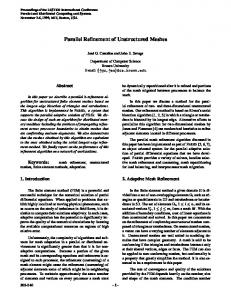
The basic idea of the Intercept method is to refine each element in only one direction, the x or y direction, depending on the location of the intersection points. We then find intersections between new lines in the refined direction and the contour line and finally simply connect the intersection points [1]. Since each refined line is horizontal or vertical (i.e. parallel to the x or y axis), pe (x, y) reduces to a univariate cubic polynomial (along the refined line). For a triangular mesh, since we employ the PCI, the following strategy can be applied Connect the two intersection points by a line and then consider some regular spaced points on this line. Draw perpendicular lines to this line at the considered points and then find the intersections between these perpendicular lines and the contour curve and connect the intersection points. Figure 16 illustrates how this strategy approximates the contour line with a refinement of eight.

0.59 0.58 0.57 0.56 0.55 0.54 0.53 0.52 0.51 0.5 0.49

0.52

0.54

0.56

0.58

0.6

0.62

0.64

Figure 16: The contour curve created by the basic Intercept method. The points on the contour curve are the intersections between the contour curve and refinement lines. The interpolant used for this problem, pe (x, y), is the Pure Cubic Interpolant (PCI) of the form

pe (x, y) = SCT = ( s3

s2

0  0 s 1) 0 c03 

16

0 0 c12 c02

0 c21 c11 c01

 3 c30 t c20   t2   . c10 t c00 1

Although the refined lines are not necessary horizontal or vertical (i.e., parallel to the x or y axis), the polynomial for each refined line will be a cubic univariate since the PCI is of total degree three. For each arbitrary line we have s = at + b and if we replace s with at + b, we will have  0 0   0    0  t3  0   t2  pe (x, y) = ( a3 3a2 b a2 3ab2 2ab a b3 b2  , 0  t  c30  1  c20   c10 c00 (8) and pe (x, y) will be a cubic univariate polynomial. Then for determining the intersections between a refined line and the contour curve with contour level v, we should find the roots of c30  0   c21   0   0 b 1)  c12   0   0  0 c03 

0 c30 c20 0 c21 c11 0 0 c12 c02

0 0 0 c30 c20 c10 0 c21 c11 c01

k3 t3 + k2 t2 + k1 t + k0 = v,

(9)

where c30  0   c21   0   0 1)  c12   0   0  0 c03 

( k3

k2

k1

k0 ) = ( a 3

3a2 b a2

3ab2

2ab

a

b3

b2

b

0 c30 c20 0 c21 c11 0 0 c12 c02 (10)

This strategy works properly as long as there is only one intersection between each refined line and the contour curve. Bradbury and Enright addressed this difficulty and showed a simple example where the whole contour curve lies inside of one element [1]. We will not encounter this situation because in our algorithm there will be exactly two intersections between the contour curve and a triangle containing a part of the contours. We might still have the situation where there is more than one intersection between a refined line and the contour curve. Note that the PCI can find at most three intersections. Figure 17(a) shows a simple situation and Figure 17(b) shows the result of our basic approach. As can be seen, we lose some sections of the contour curve due to the fact that 17

0 0 0 c30 c20 c10 0 c21 c11 c01

 0 0   0   0   0  . 0   c30   c20   c10 c00

−0.06

−0.06

−0.07

−0.07

−0.08

−0.08

−0.09

−0.09

−0.1

−0.1

−0.11

−0.11

−0.12

−0.12

−0.13

−0.13

−0.14

−0.14

−0.15 −0.16

−0.15

−0.14

−0.13

−0.12

−0.11

−0.1

−0.09

(a) True contour curve.

−0.08

−0.15 −0.16

−0.07

−0.15

−0.14

−0.13

−0.12

−0.11

−0.1

−0.09

−0.08

−0.07

(b) The contour curve plotted by the basic Intercept method.

Figure 17: An illustration of the difficulty that can arise with the basic Intercept method. function recAddMiddlePoint(p1 ,p2 ,cnt,· · ·) pm ← the middle point of p1 and p2 m1 ← the slope of the tangent line of the contour curve at p1 m2 ← the slope of the tangent line of the contour curve at p2 2 m ← m1 +m 2 p ← the intersection between the contour curve and the line passing pm with a slope m if cnt > 0 pL ← recAddMiddlePoint(p1 ,p,cnt-1,· · ·) pR ← recAddMiddlePoint(p,p2 ,cnt-1,· · ·) return pL + p + pR else return p end if end function Figure 18: The recursive algorithm to find middle points. the refinement is performed only between two intersections. On the other hand, refining the area outside of two intersections does not solve this difficulty because there is more than one intersection and it is not obvious how the intersection points should be connected. In order to resolve this difficulty, we introduce a recursive approach that attempts to find some equally spaced points located along the contour curve. The idea is to first find the middle point of the contour curve between the initial two interception points and consider this point as one of the refined points (known to be on the contour curve) and then recursively treat each of two new intervals (the intervals between the new point and each of the initial points). Figure 18 presents a more detailed description of this approach. If n is the 18

−0.06

−0.07

−0.08

−0.09

−0.1

−0.11

−0.12

−0.13

−0.14

−0.15 −0.16

−0.15

−0.14

−0.13

−0.12

−0.11

−0.1

−0.09

−0.08

−0.07

Figure 19: The contour curve created by the improved Intercept method using a fixed number of recursions to control the spacing. −0.06

−0.07

−0.08

−0.09

−0.1

−0.11

−0.12

−0.13

−0.14

−0.15 −0.16

−0.15

−0.14

−0.13

−0.12

−0.11

−0.1

−0.09

−0.08

−0.07

Figure 20: The contour curve created by the final Intercept method using a threshold value to control the spacing. number of recursive levels, we will have 2n + 1 points (including the two initial points) all lying on the contour curve. Figure 19 illustrates how this approach draws contour curves by applying a three-level recursion. An important advantage of this approach is that it locates almost equally spaced points on the contour curve. However, there is still a remaining difficulty. As can be seen in Figure 19, although the points are located equally spaced inside of each triangle, they are not totally equally spaced if we consider all triangles. In other words, the number of extra points 19

should not be equal for all triangles. For example in Figure 19, the number of extra points (7 points) is not enough for the left triangle but more than enough for the right triangle. In order to overcome this deficiency, instead of having a fixed level of recursion for all triangles, we consider a threshold for the distance between the extra points and try to locate the extra points such that the distance between each two points is less than the desired threshold. Figure 20 illustrates the effect of considering a threshold instead of the same level of recursion for all triangles. The value of the threshold can be specified by the user. 4.3.2

The Simple ODE Method (SODE)

The contouring problem can be characterized as an initial value problem [1]. The problem for the contour level v is to solve u(x, y(x)) = v,

(11)

where y is a function of x. If we differentiate both sides of this equation with respect to x, we obtain ux (x, y(x)) + uy (x, y(x)) · yx (x) = 0, or yx (x) = −

ux (x, y(x)) . uy (x, y(x))

(12)

(13)

This ODE is satisfied for (x, y(x)) lying on the contour curve. If we consider x as a function of y, we can similarly derive xy (y) = −

uy (x(y), y) . ux (x(y), y)

(14)

We can approximate u(x, y),ux (x, y) and uy (x, y) at prescribed values of x and y using the PCI (and its partial derivatives). We can then solve equation (13) or (14) by applying a numerical IVP solver starting from a known intersection point. Furthermore, rather than applying an IVP solver, we can compute approximations to y(x) and yx (x) (or x(y) and xy (y)) at prescribed values directly from the PCI. We can then interpolate the contour curve by using an appropriate order Hermite interpolant. The minimum number of extra points (in addition to the intersection points) necessary to define the Hermite interpolant is dependent on the contour curve and some properties of the two intersection points. Bradbury and Enright considered one middle point for all situations [1]. However, for some situations that can arise, we need no middle point and the contour curve can be approximated accurately with only the two intersection points. In the case that the gradient of u at the two intersection points has the same sign (for both x and y directions), we need no middle points and the contour curve can be computed precisely by applying a cubic Hermite interpolant. Figure 21 shows such a situation. For the other cases, we will use the approach 20

that will be introduced in the next method, the ODE with arclength. When the magnitude of the respective derivative, (yx or xy ), is much larger than one, the Hermite interpolant may not approximate the solution of this IVP very well. We apply the ODE with arclength method for such situations as well.

0.1 0.08 0.06 0.04 0.02 0 −0.02 −0.04 −0.06 −0.08 −0.1 −0.1

−0.05

0

0.05

0.1

Figure 21: The common situation in contour curves.

−0.06

−0.06

−0.07

−0.07

−0.08

−0.08

−0.09

−0.09

−0.1

−0.1

−0.11

−0.11

−0.12

−0.12

−0.13

−0.13

−0.14

−0.15 −0.16

−0.14

−0.15

−0.14

−0.13

−0.12

−0.11

−0.1

−0.09

(a) True contour curve.

−0.08

−0.15 −0.16

−0.07

−0.15

−0.14

−0.13

−0.12

−0.11

−0.1

−0.09

−0.08

−0.07

(b) The contour curve plotted by the ODEA method with no middle point.

Figure 22: A situation where the ODEA method fails if no middle point is considered.

21

−0.06

−0.07

−0.08

−0.09

−0.1

−0.11

−0.12

−0.13

−0.14

−0.15 −0.16

−0.15

−0.14

−0.13

−0.12

−0.11

−0.1

−0.09

−0.08

−0.07

Figure 23: The contour curve plotted by the ODEA method with one middle point. 4.3.3

The ODE with Arclength Method (ODEA)

In the SODE method, we assumed that y is a function of x (or x is a function of y). An alternative method is to parameterize with respect to arclength and assume both x and y to be functions of arclength [1]. In this case, we will have u(x(s), y(s)) = v,

(15)

where v is the contour level and s is the arclength. Then if we differentiate (15) with respect to s, we will obtain ux · xs + uy · ys = 0,

(16)

and if we consider a normalization condition for the arclength, we will get xs 2 + ys 2 = 1.

(17)

From equations (16) and (17) we will obtain a system of ODEs, ±uy xs = p , ux 2 + uy 2

(18)

∓ux , ys = p ux 2 + uy 2

(19)

which is satisfied on the contour curve. Note that the sign of xs (±) differs from the sign of ys (∓). In other words, if xs and uy have the same sign, ys and ux should have different sign and vice versa. In order to identify the proper sign in equations (18) and (19), an intersection test can be done along a single 22

line of refinement. Like the SODE approach, we can obtain approximations of x(s), y(s), xs (s) and ys (s) at each arbitrary point directly from the PCI using Hermite interpolation to approximate x(s) and y(s) separately. In most cases, the data (x(s), xs (s), y(s) and ys (s)) from two intersection points is adequate to accurately approximate the contour curve. However in some cases, the Hermite interpolants fail to determine a suitable approximation and at least one extra point is required. Figure 22(a) illustrates one of these situations and Figure 22(b) shows the result of the Hermite interpolant if we apply it with only the two intersection points. By analyzing the difficulty and observing the result of some special situations, we realized that if either x(s) or y(s) has more than one extreme point on the contour curve, the Hermite interpolant may fail to accurately interpolate the contour curve. Note that since the PCI is of degree 3 in x and y, the corresponding polynomial can have at most two extreme points in each direction x or y (corresponding to one minimum and one maximum). We can assume that the middle point of the contour curve locates these two extreme points in two different sections. In order to find the middle point of the contour curve, a similar approach to that employed in the SODE method can be used. After identifying the middle point we can use two cubic Hermite interpolants for computing the contour curve. Figure 23 illustrates the result of the situation corresponding to Figure 22 when we consider the middle point. One advantage of the ODEA method is its relationship to Hermite interpolation of the exact contour curve. As we mentioned in the previous section, the Hermite interpolant fails to approximate the solution of the associated IVP (13) or (14) accurately if the derivative is much larger than one in magnitude. However, for the ODEA method, due to the normalization condition, it is guaranteed that xs and ys are both bounded by one in magnitude. Since the ODEA method needs fewer middle points than the Intercept method, it computes contours much faster than the Intercept method. However, its results may not be as precise as those of the Intercept method since it is approximating the contours of the underlying Hermit interpolant of the contour curve. In order to obtain more accurate results with the ODEA method, we can add some extra ‘middle points’ and then apply a piecewise cubic Hermit defined over a finer mesh to compute the contour curve. We call this method, the Alternate ODE with Arclength method (AODEA). Like with the Intercept method, the user can specify a threshold value δ as the minimum distance separating neighbor points. For the intercept method the contribution to the error in the contour segment will be O(δ 2 ) while, for the AODEA method the contribution to this error will be O(δ 4 ). The appropriate threshold value for use with AODEA will therefore be larger than that for the Intercept method.

5

Experimental Results

In this section, we will first introduce a test problem. We will then present test results comparing our three fast contouring algorithms with other contouring

23

methods. We consider a single test problem to illustrate the relative performance of the three fast contouring algorithms and to confirm that the observed performance is consistent with the theory. The problem has a known closed-form solution and we use this known solution to generate the required data at the unstructured mesh points. The test problem is (5−10x)2 (5−10y)2 (5−10y)2 ∂u ∂ 2 u − = (50 − 100y)(0.75e(− 2 ) + 0.75e(− 2 ) e(− 2 ) ) + 2 ∂y ∂x

100(e(−

(5−10x)2 2

)

+ 0.75e(−

(5−10x)2 2

) (−

e

(5−10y)2 2

)

) − (50 − 100x)ux (20)

and its closed-form solution is u(x, y) = e(−

(5−10x)2 2

)

+ 0.75e(−

(5−10y)2 2

)

+ 0.75e(−

(5−10x)2 2

) (−

e

(5−10y)2 2

)

.

(21)

Figure 24 shows its surface and contour plots. 1

0.9

0.8

0.7

0.6 2.5

0.5

2 1.5

0.4

1 1 0.5

0.3

0.8 0 1

0.2

0.6 0.8 0.4

0.6 0.4

0.1

0.2 0.2 0

0

0

(a) The surface plot

0

0.1

0.2

0.3

0.4

0.5

0.6

0.7

0.8

0.9

(b) The contour plot

Figure 24: Test problem: The surface plot and the contour plot. We have compared our fast contouring algorithms, introduced in section 4, with the Matlab contour procedure and those addressed by Bradbury and Enright in [1]. In order to compare the methods, a uniform distribution of the data is considered because the Matlab contour procedure needs the data on a rectangular mesh. It should be acknowledged the Matlab contour procedure is more general since our contouring algorithms are based on the availability of the PCI which needs to know the underlying PDE. Both contouring algorithms implemented by Bradbury and Enright, FCINT and FCODE, are included for comparison [1]. Table 1 shows the average error of applying the methods on a rectangular mesh with different number of mesh points. For each segment of the approximate contour curve that lies in a mesh element, a random point on 24

1

the curve is considered as a sample point. Therefore the total number of sample points depends on the size of the underlying mesh and the number of contour curves. The error reported, for each sample point, is the absolute difference between the true value of u(x, y) and the value of the contour curve. In addition, Table 2 shows the corresponding required computer time. From Tables 1 and 2, it can be inferred that our algorithms can be both more accurate and faster than the Matlab contour procedure, FCINT and FCODE. Although the Intercept method is not as accurate as the SODE and ODEA methods for this rectangular mesh, it was more accurate than the others for the unstructured triangular meshes we investigated. However the total required time for the Intercept method is more. Tables 3 and 4 show the average error and corresponding required time of applying our fast contouring algorithms on an unstructured triangular mesh with 900, 1600 and 2500 mesh points. In section 4, an alternate ODEA algorithm, the AODEA, was introduced to improve the accuracy of ODEA method. The results of the AODEA method are also presented in Tables 3 and 4. As can be seen, the AODEA method is more accurate than the ODEA but needs more time as well. The accuracy of the AODEA method can be controlled by the value of the applied threshold. Figure 25 shows the contour plots generated by the Intercept method on unstructured triangular meshes with 900 and 2500 mesh points. The plots for the other methods are the same and visually indistinguishable. # Mesh Points 30*30 40*40 50*50

Matlab 0.3066 0.4522 0.4605

FCINT 0.001900 0.000741 0.000273

Algorithm FCODE Intercept 0.002300 0.00001270 0.000811 0.00000798 0.000234 0.00000766

SODE 0.00001060 0.00000291 0.00000213

ODEA 0.00001010 0.00000235 0.00000183

Table 1: Average error for the different methods for a rectangular mesh with 30*30, 40*40 and 50*50 mesh points.

# Mesh Points 30*30 40*40 50*50

Matlab 14.66 23.18 35.40

FCINT 9.78 17.19 22.08

Algorithm FCODE Intercept 9.50 9.61 16.59 13.40 21.75 18.95

SODE 5.33 9.33 14.77

ODEA 5.54 9.50 15.21

Table 2: Total required time (in terms of seconds) for the different methods for a rectangular mesh with 30*30, 40*40 and 50*50 mesh points.

25

# Mesh Points 900 1600 2500

Intercept 0.00000903 0.00000655 0.00000546

Algorithm SODE ODEA 0.000687 0.000687 0.0000299 0.0000226 0.0000128 0.0000123

AODEA 0.0000247 0.0000156 0.00000663

Table 3: Average error for the different methods for an unstructured triangular mesh with 900, 1600 and 2500 mesh points. # Mesh Points 900 1600 2500

Intercept 10.98 14.11 18.35

Algorithm SODE ODEA 5.43 5.55 9.28 9.39 13.62 13.79

AODEA 6.65 10.49 15.54

Table 4: Total required time (in terms of seconds) for the different methods for an unstructured triangular mesh with 900, 1600 and 2500 mesh points.

1

1

0.9

0.9

0.8

0.8

0.7

0.7

0.6

0.6

0.5

0.5

0.4

0.4

0.3

0.3

0.2

0.2

0.1

0.1

0

0

0.1

0.2

0.3

0.4

0.5

0.6

0.7

0.8

0.9

1

(a) Intercept (900 points)

0

0

0.1

0.2

0.3

0.4

0.5

0.6

0.7

0.8

0.9

(b) Intercept (2500 points)

Figure 25: The contour plots of the test problem generated by the Intercept method on triangular meshes with 900 and 2500 mesh points.

6

Conclusions

In this investigation we have focussed on improving the accuracy and efficiency of existing contouring algorithms. We have not considered how best to address known difficulties such as the detection (and avoidance) of intersecting contour segments or the effect on the contour segments of “local saddle points” (associated with the specified contour level). These difficulties are a challenge for 26

1

any contour algorithm and the effective handling of them will be left for future study. We introduced three fast contouring algorithms based on the PCI. These contouring algorithms were compared to the built-in Matlab contour procedure and the contouring algorithms introduced by Bradbury and Enright. For rectangular meshes, we demonstrated that our algorithms can be both more accurate and faster than the others. We also showed that they are fast and accurate for unstructured data sets. Among our algorithms, the ODEA method is much faster than the Intercept method. However, it may not compute contours as accurate as the Intercept method. We therefore modified this approach and introduced the AODEA method to obtain more accurate results at a modest increase in the required computer time.

7

Acknowledgement

The authors would like to thank the referees for their helpful suggestions and comments.

References [1] Emma L. Bradbury and Wayne H. Enright. Fast contouring of solutions to partial differential equations. ACM Transaction on Mathematical Software, 29(4):418–439, December 2003. [2] Wayne H. Enright. Accurate approximate solution of partial differential equations at off-mesh points. ACM Transaction on Mathematical Software, 26(2):274–292, June 2000. [3] MathWorks. MATLAB online documentation, 12 edition. [4] Hassan Goldani Moghaddam. Efficient contouring on unstructured meshes. Master’s thesis, University of Toronto, 2004. [5] Hassan Goldani Moghaddam and Wayne H. Enright. The PCI: A Scattered Data Interpolant For the Solution of Partial Differential Equations. In Proceedings of International Conference on Adaptive Modeling and Simulation, ADMOS 2005, Barcelona, Spain, September 2005.

27