efficient convex optimization for engineering design 0 - Stanford ...

EFFICIENT CONVEX OPTIMIZATION FOR ENGINEERING DESIGN Stephen Boydy, Lieven Vandenberghez , Michael Granty

y Information Systems Laboratory, Stanford University, Stanford, California z Electrical Engineering Department, K.U. Leuven, Leuven, Belgium

Abstract. Many problems in engineering analysis and design can be cast as convex

optimization problems, often nonlinear and nondierentiable. We give a high-level description of recently developed interior-point methods for convex optimization, explain how problem structure can be exploited in these algorithms, and illustrate the general scheme with numerical experiments. To give a rough idea of the eciencies obtained, we are able to solve convex optimization problems with over 1000 variables and 10000 constraints in around 10 minutes on a workstation.

Keywords. Optimization, numerical methods, linear programming, optimal con-

trol, robust control, convex programming, interior-point methods, FIR lter design, conjugate gradients 1. INTRODUCTION Many problems in engineering analysis and design can be cast as convex optimization problems, i.e., min f0 (x) s.t. fi (x)  0; i = 1; : : :; L; where the functions fi are convex. It is widely known that such problems have desirable properties, e.g., locally optimal solutions are globally optimal. In fact much more is true | roughly speaking, convex optimization problems are fundamentally tractable, both in theory and in practice. In this paper we consider the convex optimization problem min cT x (1) s.t. F(x)  0; where
F(x) = F0 + x1F1 +


+ xm Fm :

The problem data are the vector c 2 Rm and m + 1 symmetric matrices F0; : : :; Fm 2 Rnn. The inequality sign in F(x)  0 means that F(x) is positive semide nite. We call problem (1) a positive de nite program or PDP. Although the PDP (1) may appear quite special-

ized, it includes many important problems as special cases. For instance, consider the linear program (LP) min cT x (2) s.t. Ax + b  0 where the inequality denotes componentwise inequality. Since a vector v  0 (componentwise) if and only if the matrix diag(v) (the diagonal matrix with the components of v on its diagonal) is positive semide nite, we can express the linear program (2) as a PDP with F(x) = diag(Ax+b), i.e., F0 = diag(b); Fi = diag(ai ); i = 1; : : :; m; where ai is the ith column of A. Many other problems, including most of the convex optimization problems encountered in engineering, can be written as PDPs. Positive de nite constraints also arise directly in a number of important applications, for example, in control and system theory (Boyd et al. 1994, Boyd and Barratt 1991). Positive de nite programming therefore offers a uni ed way to study the properties of, and derive algorithms for, a wide variety of convex optimization problems. Most importantly, however, PDPs can be solved very eciently using recently developed interior-point methods. Interior-point methods were rst introduced for

linear programming by Karmarkar in 1984 (Karmarkar 1984). Although controversial at the time, it is now generally accepted that interiorpoint methods for LPs are competitive with the simplex method, and even faster for large problems. An important breakthrough took place in 1988, when Nesterov and Nemirovsky generalized interior-point methods for LP to general convex programming (Nesterov and Nemirovsky 1994). The experimental results reported in this paper were obtained using a primal-dual potential reduction method. The method is based on the method described by Nesterov and Nemirovsky (Nesterov and Nemirovsky 1994; x4.5), which generalizes Ye's method for linear programming (Ye 1991). We modify this basic interior-point method by using conjugate gradients to exploit problem structure, as explained in (Vandenberghe and Boyd 1993). We give a brief description of the method in the next two sections. For more details, see (Vandenberghe and Boyd 1994). In x4 we show how to exploit problem structure, and in x5 we apply these techniques to three (families of) engineering problems. 2. DUALITY The dual problem associated with the PDP (1) is max ,TrF0Z s.t. TrFi Z = ci ; i = 1; : : :; m Z  0: = ZT

(3)

2 Rnn,

Here the variable is the matrix Z and TrX denotes the trace of the matrix X.

Under mild conditions, the optimal values of the primal problem (1) and the dual problem (3) are equal (Rockafellar 1970). This fact has important consequences.  Every dual feasible Z (i.e., every matrix Z that satis es the constraints in (3)), proves a lower bound ,TrF0 Z on the optimal value of the PDP (1).  If F(x)  0, and Z is dual feasible, then the dierence between the primal and the dual objective values is nonnegative, cT x + TrF0Z  0: We call the quantity on the left the duality gap of the pair (x; Z).  If the duality gap is zero, then x and Z are optimal points, solving the primal PDP (1) and the dual (3). Primal-dual interior-point methods generate a se-

quence of primal and dual feasible points x(k) and Z (k) , where k = 0; 1; : : : denotes iteration number. We can interpret x(k) as a suboptimal point and Z (k) as a certi cate that proves the lower bound ,TrF0 Z (k) on the optimal value. The iteration is terminated if the duality gap cT x(k) + TrF0Z (k) becomes less than a pre-speci ed tolerance . 3. ALGORITHM The interior-point method is based on a potential function '(x; Z). The essential properties of the potential function are:  ' is smooth on the interior of the feasible set, and in nite outside the feasible set.  The duality gap is less than  exp '(x; Z), where  is a positive constant; in particular, if '(x; Z) ! ,1, then (x; Z) approach optimality. At each iteration of the algorithm, the potential function decreases by at least a xed amount: '(x(k+1); Z (k+1))  '(x(k+1); Z (k+1)) , ; where is an absolute constant. As a consequence, the iterates remain feasible, and converge to the optimum. The duality gap converges to zero exponentially. For the PDP (1), we use the potential function '(x; Z) =
q log(cT x + TrF0 Z) + log det F(x),1 + log det Z ,1 :

(4)

The rst term (4) rewards a decrease in the duality gap. The second and third terms act as barrier functions that keep F(x) and Z positive de nite. The scalar q is a parameter that controls the relative weight of the dierent terms. The updates x(k+1), Z (k+1) are generated from x(k), Z (k) as follows. A suitable pair of search directions, x, Z, are found by (approximately) solving a least-squares problem. Then, primal and dual step lengths  and are chosen to (approximately) minimize the potential '(x(k) + x; Z (k) + Z) in the plane de ned by the current points and the search directions. This is called the plane search. We then set x(k+1) = x(k) + x, Z (k+1) = Z (k) + Z, and repeat the process. 4. CONJUGATE GRADIENTS One of the most remarkable properties of interiorpoint methods is their insensitivity to problem size. The number of iterations increases very slowly, typically as the logarithm of the problem

size. For most practical purposes, the number of steps can be considered to be almost independent of the dimension. Typical numbers range from 10 to 50. The overall computational eort is therefore determined by the amount of work per iteration. Skipping details, we can say that the main eort in every iteration is the solution of a least-squares problem of the form min v 2 Rm



(k)

D

,

m X i=1



vi S (k) Fi S (k)

F

(5)

to compute suitable search directions. Here, k
kF denotes the Frobenius norm, i.e., ,




kAk2F = Tr AT A =

X

i;j

A2ij :

As the superscripts suggest, the matrices D(k) = D(k)T and S (k) = S (k)T in (5) change every iteration. As a practical guideline, therefore, the total complexity of solving a convex problem is equal to the work of solving a relatively small (say, 10{ 50) and almost constant number of least-squares problems of the form (5). Problem (5) has m variables and n(n+1)=2 equations. Using direct methods it can be solved in O(m2 n2 ) operations. Important savings are possible when the matrices Fi are structured. The easiest type of structure to exploit is block-diagonal structure. Assume F(x) consists of L diagonal blocks of size ni, i = P 1; : : :; L. Then the number of equations in (5) is Li=1 ni(ni + 1)=2, which is often an order less than n(n + 1)=2. For instance, in the LP case (diagonal matrix F(x)), the number of variables is n, and solving the least-squares problem requires only O(m2 n) operations. Usually much more can be gained by exploiting the internal structure of the diagonal blocks in Fi . The conjugate gradients method or the LSQR algorithm of Paige and Saunders (Paige and Saunders 1982) appear to be very well suited. In exact arithmetic, these algorithms solve (5) in m + 1 iterations, where each iteration requires one evaluation of the `forward' mapping, (v1 ; : : :; vm ) 7!

m X i=1

vi Fi ;

(6)

and one evaluation of its adjoint W 7! (TrF1 W; : : :; TrFm W)

(7)

for some vector v and symmetric matrix W = W T . When the matrices Fi are unstructured, these two operations take mn2 operations. Hence,

the cost of solving (5) using LSQR is O(n2 m2 ), and nothing is gained over direct methods. In most cases, however, the two operations (6) and (7) are much cheaper than mn2 because of the special structure of the matrices Fi . A wellknown example is a sparse LP, but sparsity is not the only example. The equations are often dense, but still highly structured in the sense that the mappings (6) and (7) can be evaluated faster than O(mn2 ) operations. We will see several examples in x5. In practice, i.e., with roundo error, the standard conjugate gradients algorithms can perform quite poorly; the number of iterations required to solve the least-squares problem can be much higher than m + 1. Two techniques can be used to improve the rate of convergence. The standard technique is pre-conditioning, described in (Golub and Loan 1989). There is no simple universal method for constructing a suitable pre-conditioner, but often a good choice follows from the properties of the underlying engineering problem. The design of a pre-conditioner is problem dependent; the engineer's experience with and intuition about the problem is invaluable. The other technique is re-orthogonalization. Reorthogonalizaton can always be applied. It makes the algorithm converge as in exact arithmetic (i.e., in O(m) steps), but is expensive: it increases the cost of N LSQR iterations with O(mN 2 ) operations. This is too expensive if the algorithm is run to completion. This brings us to another great advantage of using iterative methods to solve the least-squares problem (5): the option of early termination. The LSQR-algorithm produces good search directions even if the iteration is stopped before the exact solution of the least-squares problem (5) has been found. It can be proved that early termination does not aect the worst-case convergence rate, provided a good stopping criterion is used (Vandenberghe and Boyd 1993). In our experience, we often nd that suitablepsearch directions can be generated after only O( m) LSQR iterations. An important consequence is that the cost of reorthogonalization is not nearly as high as it is when LSQR is run to completion, i.e., O(m) iterations. We should mention one important issue that arises when early termination of LSQR is used. When the least-squares problem (5) is solved exactly, the dual search direction Z is computed from its residual. With early termination of LSQR, this search direction will not exactly satisfy the equality constraints TrFi Z = 0 required for dual fea-

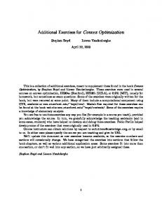
sibility. The user must supply a subroutine that perturbs a dual search direction that nearly satis es these equalities into one that exactly satis es them. The design of this subroutine is problemdependent; see (Vandenberghe and Boyd 1993). Let us summarize the main points. Many convex optimization problems arising in engineering can be cast in the form of the PDP (1). Roughly speaking, solving the PDP (1) requires the (approximate) solution of between 10 and 50 leastsquares problems of the form (5). Using LSQR to approximately solving such a least-squares p problem requires somewhere between O( m) and O(m) evaluations of the forward and adjoint mappings (6) and (7). It follows that if we can exploit problem structure to evaluate these mappings ef ciently, we can solve the PDP (1) eciently. This general scheme is summarized in Figure 1. can evaluate forward, adjoint fast

(exploiting structure)

+ can solve least-squares problem fast

(using LSQR)

+ can solve convex problem fast

(using interior-point methods)

Fig. 1. Exploiting problem structure to eciently solve convex problems.

immediately point out that LSSOL was not designed to exploit structure; we are merely comparing INTPT, an interior-point code that exploits problem structure, to LSSOL, an optimized simplex-based LP code that does not exploit structure. We should also point out that INTPT is still in development, and that no eort was expended in optimizing it for these examples. For instance, we used no pre-conditioning at all. 5.1 Testing environment

We used a DECstation 5000/240 with 64 megabytes of memory. DEC Fortran version 3.2 was used to compile LSSOL and the Fortran subroutines employed by INTPT; the GNU Foundation's g++ was used to compile the C++ code. Full compiler optimization was enabled in all cases. We used the standard UNIX library routine getrusage to measure the total execution time, t(M), and the amount of resident (in-core) memory usage, m(M), for a given number of variables M. We collected data for a wide range of problem sizes, in an attempt to measure the general trends of each. The execution time t(M) was t to a function of the form ~t(M) = a + bM c by minimizing X

i

(log(a + bMic ) , logt(Mi ))2

over a, b, and c. Likewise, the memory consumption was t to m(M) ~ = a + bM + cM 2 by minimizing X

5. EXPERIMENTAL RESULTS In this section we illustrate the general scheme outlined above on three (convex) engineering problems. The rst problem is FIR lter design. The second is a robust input design problem: we must determine an input that will work well with multiple, given plants. The third problem is robust input design for a multiple-input multipleoutput plant. In each case we generate a family of problems indexed by a dimension M which is the number of free variables in the problem. Michael Grant developed the software, called INTPT below, as well as the examples. Even though INTPT handles general PDPs, these three examples are in fact LPs. This allows us to compare the computational eort and memory usage of INTPT with that of LSSOL, a widely used package for solving linear and linearly-constrained quadratic programs (Gill et al. 1986). We must

(8)

i

(a + bMi + cMi2 , m(Mi ))2

(9)

over a, b, and c. These curves are included in the plots presented below. The constant factor in m(M) ~ was subtracted from the data before plotting, in order to remove the contributions of the programs themselves and to better show the actual growth rates on a logarithmic plot. 5.2 FIR lter design

Suppose we wish to design a (non-causal) zerophase lter which satis es a set of frequency response constraints while minimizing its peak impulse response. We focus on the Type I low-pass case, a symmetric lter with 2L+ 1 taps, and frequence response H(f) =

L X k=,L

h(k)e,j 2kT f s

k=1

2h(k) cos(2kTsf)

Other lter design problems follow similarly. Given a desired frequency response Hr (f) and permissible deviation
(f), we might specify the design problem as min max jh(k)j s:t: jH(fi ) , Hr (fi )j 
(fi ) (10) i = 1; : : :; N; k = 0; : : :; L; where the fi s denote frequencies of interest within the passband and stopband of the lter. The unknowns are the coecients h(0), : : :, h(L). We can write (10) as an LP (2) by introducing a new variable w: min w s:t: ,w  h(k)  w; k = 0; : : :; L
(fi )  H(fi ) , Hr (fi ) 
(fi ) i = 1; 2; : : :; N: This LP is very structured. In order to evaluate the forward mapping associated with the constraints, we need to compute the frequency response of the lter, given a set of coecients h(k). This can be done very eciently using the Fast Fourier Transform (FFT). The adjoint mapping can be computed very eciently using the inverse FFT. To generate example problems of various sizes, we began with the following speci cation of a continuous-time, zero-phase FIR low-pass lter: min khk s:t: h(t) = h(,t) h(t) = 0 t > 1sec (11) jH(f) , 1j < 0:01 f  4Hz jH(f)j < 0:01 f  8Hz where khk denotes the l1 or peak norm of the

impulse response h. The impulse response of the optimal lter is shown in Figure 2. Discrete approximations to this problem were created by assuming a piecewise-linear impulse response with 2M evenly-spaced segments. This is equivalent to a 2M ,1-tap FIR lter (M unique taps) with a triangle hold at the output. The frequency-response constraints were discretized at 4M +1 frequencies and compensated to include the contribution of the triangle-hold response. The result was a linear program with M + 1 variables and 10M + 2 constraints. INTPT exploited the structure of this problem by using a mixed-radix, fast discrete cosine transform (DCT) to evaluate the frequency-response

4 3 2 Amplitude

L X

1 0 -1 -2 -3 -1

-0.8

-0.6

-0.4

-0.2

0 0.2 Time, seconds

0.4

0.6

0.8

1

0

10

-1

10 Magnitude

= h(0) +

-2

10

-3

10

0

1

10

2

10 Frequency, Hz

10

Fig. 2. The impulse response and frequency response of the optimal lter. constraints. We chose problem sizes for which the DCT was most ecient, so the evaluation time of the forward and adjoint operators was reduced by a factor of O(M= log M). To obtain 4M + 1 frequencies from the DCT we padded the M unique taps with 3M + 1 zeros; yet despite this apparent waste, the logarithmic growth of the DCT's complexity still yielded big gains. The plots in Figure 3 compare the execution times and data size, respectively, of the two solvers for various problem sizes. In this case, the advantage in both execution time and memory consumption lies solely with INTPT. The execution time grew as O(M 1:67) for INTPT and O(M 3:28) for LSSOL. The largest problem solved had over 1000 (independent) variables (over 2000 taps in the FIR lter) and 10000 constraints. INTPT solved this problem in about 4 minutes, using about 4Mb of memory. 5.3 Robust open-loop input design

In the open-loop input design problem , we are given a discrete-time linear system with input u(k) 2 Rn and output y(k) 2 Rn . The problem is to design an input trajectory that makes the output track a given reference signal ydes (k). For example, one may want to minimize the peak i

o

tracking error



y(k) , ydes (k) : max 1 k

some of these constraints is

5

10

LSSOL INTPT

Execution time, seconds

3

10

2

10

1

10

0

10

-1

10 5 10

Memory consumption, kilobytes



(i)

min max

y (k) , ydes (k) i;k 1 s.t. 0  uj (k)  umax juj (k + 1) , uj (k)j  smax (13) the state equations (12) x(i) (0) = 0 0  k < N; 1  i  L; j = 1; : : :; ni:

4

10

The variables are the input vectors u(k), k = 0; : : :; N , 1.

4

10

3

10

2

10

1

10 1 10

2

10 Number of variables

3

10

Fig. 3. Execution times and memory consumption for the lter design example.

The robust input design problem involves multiple plants x(i) (k + 1) y(i) (k)

(i) x(i)(k) + ,(i) u(k) H (i) x(i)(k) + J (i) u(k);

= (12) = for i = 1; : : :; L. The same input is applied to each plant. The purpose is to design an input trajectory that works well for all plants simultaneously, e.g., by minimizing the maximum of the peak tracking errors



(i) des max

y (k) , y (k) : i;k 1

We can also take into account various convex constraints on inputs and outputs, e.g., limits on the input amplitude,

ku(k)k1  umax ; slew rate constraints on the input,

ku(k + 1) , u(k)k1  smax ; or envelope bounds on the output, ymin  yj (k)  ymax : A convex optimization problem that includes

Again, problem (13) can be written as an LP with very structured equations. To evaluate the forward mapping associated with the constraints, we need to compute the output vectors y(i) (k) for a given input trajectory u(k), k = 0; : : :; N ,1. This can be done very eciently by directly simulating the linear systems (12). The adjoint mapping can be evaluated by simulating the adjoint linear systems (Kailath 1980). This reduces the calculation time for the linear operators from O(N 2 ), if no structure is exploited, to O(N). In the experiment we take two single-input singleoutput systems, obtained from the continuoustime systems H1(s) = 16=(s2 + 1:2s + 16) H2(s) = 25=(s2 + 1:2s + 25) using a rst-order hold on the input, with sampling interval
T = 5=M, over the time interval 0  t  5. The input is constrained to lie between zero and one. The maximum slew rate is 1.25/sec. The reference trajectory is piecewise linear: zero for 0  t  2, one for 3  t  5, with a linear transition (slew) between t = 2 and t = 3. This results in an LP with M+2 variables and 10M+12 constraints. Figure 4 shows the step responses of the two systems, an optimal input u, and the resulting output trajectories. The optimal tracking error is about 0:05, which is plotted in dotted line type above and below the reference trajectory. The gures demonstrate several interesting properties of the problem. First of all, the impulse responses of the two systems often have opposite sign; consequently the optimal control inputs for the individual plants are quite dierent. Secondly, the optimal control input contains the very interesting \preparatory" behavior for t  1 that standard control input design strategies would not suggest. The plot in Figure 5 compares the execution time and memory consumption of the two methods for various problem sizes. While LSSOL is faster for smaller problems, the execution time grows faster

3

2

10

LSSOL INTPT 1.5 2

Execution time, seconds

y

10 1

0.5

0

1

10

0

10

1 0.8 -1

10 u

0.6 4

10

0.4 0.2 Memory consumption, kilobytes

0

1 0.8

y

0.6 0.4

3

10

2

10

1

10

0.2 0 0

0

0.5

1

1.5

2

2.5 t

3

3.5

4

4.5

5

Fig. 4. Step responses, control input, and output trajectories, respectively, for the robust input design example. with size than for INTPT, and INTPT overtakes it at approximately M = 170. Speci cally, the execution time for INTPT grew as approximately O(M 2:2), while that for LSSOL grew as O(M 2:8). Comparing the memory consumption of the two programs exposes another signi cant dierence. LSSOL consumes a much larger amount of memory than INTPT, and those requirements grow with O(M 2 ) behavior. As a result, the largest problems exceeded our system-imposed memory usage limits; but without those limits, virtual memory paging would begin to degrade the performance of either solver. The iterative methods of INTPT, however, allow for much more modest growth in memory needs with problem size, so much larger problems can be handled. The growth does contain a small O(M 2) component, but its coecient is much smaller than for LSSOL, resulting in reasonable memory demands even for the largest problem sizes. The largest problem considered had over 1000 variables and 10000 constraints. INTPT solved it in about 15 minutes, using negligible memory (under 2Mb). 5.4 Multi-input, multi-output input design

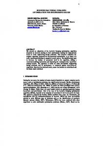
The third problum is a robust input design problem for a multi-input muti-output system. We consider a (simpli ed) model of a rapid thermal processor system, used for semiconductor manufacturing. An array of ni tungsten-halogen lamps

10 1 10

2

3

10

10

Fig. 5. Execution times and memory consumption for the robust input design example. TUNGSTEN-HALOGEN LAMP

REFLECTOR

THERMOCOUPLE POINT

WAFER HOLDER QUARTZ WINDOW

WAFER

SILICON WAFER

COLD WALL CHAMBER

Fig. 6. An experimental rapid thermal processing (RTP) con guration. is used to rapidly control the temperature of a semiconductor wafer, which for testing purposes is out tted with no thermocouples, as shown in Figure 6 (Norman 1992, Gyugyi 1993). A linearized model of the dynamics between the lamp powers and the thermocouple readings was taken from (Gyugyi 1993), in which 3 lamps and 5 thermocouples are employed. The dynamics from the lamp outputs l(t) to the thermocouple readings o(t) were described by a 5-state state-space model (; ,; H = I; J = 0) with eigenvalues ranging from -1.113 to -0.0181. A rst-order model Hlamp (s) = 8=(s + 8) was assigned to the dynamics between each lamp input ui(t) and its output li (t). We also placed hard limits on the lamp inputs, and slew-rate limits on the lamp outputs. A typical reference trajectory for rapid thermal processing involves ramping the temperature up to a desired value, holding, and then ramping back

5

2

10

LSSOL INTPT

1.5

4

Execution time, seconds

10

u

1

0.5

0

3

10

2

10

1

10

-0.5

0

-1 1.2

10 5 10

Memory consumption, kilobytes

1

0.8

y

0.6

0.4

0.2

4

10

3

10

0

-0.2 0

2

1

2

3

4

5 6 Time, seconds

7

8

9

10

Fig. 7. Control inputs and output trajectories of the MIMO control design example. down:

8 > > > >
1 3:25  t  6:75 (14) > 0:8(8 , t) 6:75  t  8 > > : 0 8  t  10 If we measure tracking error only during the time periods in which the reference trajectory is constant, and ignore the behavior during the transitions, the design problem becomes min w s:t: o(t) _ = o(t) + ,l(t) l_(t) = 8(u(t) , l(t)) ko(t)k1  w 0  t  2 ko(t) , ~1k1  w 3:25  t  6:75 (15) ko(t)k1  w 8  t  10 ,1  ui(t)  2 kl_i (t)k1  12 0  t  10 Plots of optimal control inputs and the resulting trajectories are given in Figure 7. We form an LP from this in nite-dimensional problem by assuming a zero-order hold on the inputs u, discretizing the dynamics, and sampling the constraints. Given a sampling rate
t = t=M, the result is an LP with M + 2 variables and approximately 13:5(M + 1)-constraints. Once again, using state and co-state simulation for the dynamic system, INTPT signi cantly reduced the complexity of the forward and adjoint

10 2 10

3

10 Number of variables

Fig. 8. Execution times and memory consumption for the MIMO input design example. operators used to solve the problem. The plots in Figure 8 document the signi cant performance gains made over LSSOL. The execution time grew as O(M 2:01) for INTPT and O(M 3:32) for LSSOL. The largest problem considered had over 1500 variables and 20000 constraints. INTPT solved it in about 18 minutes, using about 5Mb memory. 5.5 Future improvements

The results shown here are the rst complete tests of INTPT that have been performed. Pro ling the code reveals that there is signi cant room for problem-independent improvement in the performance of the engine which could not be incorporated into the code before the completion of this article. Therefore, we can expect that future versions of INTPT will show much improved performance. Execution pro ling has revealed that a very large component of the execution time is spent performing the reorthogonalizations in the iterative leastsquares solver. Currently, LSQR (Paige and Saunders 1982) with early termination is used to solve the least-squares problems associated with the interior-point technique, and complete reorthogonalization is used at each iteration to insure convergence. Methods of selective reorthogonalization, such as that described in (Parlett and Scott 1979), promise to greatly reduce the number of orthogonalizations performed.

For convex programs consisting primarily of linear, quadratic, and other simple nonlinear constraints, the second largest consumer of CPU time is the plane search algorithm. The plane search reduces to minimizing over  and the function f(; ) = q log(c1 + c2  + c3 )

, ,

N X i=1 N X i=1

(16)

log(1 + i ) log(1 + i )

where c1 > 0, and the constants ci , i and i are given (Vandenberghe and Boyd 1993). The current implementation uses damped Newton linesearch iterations. We are currently experimenting with rational approximations of f, which appear to greatly reduce the number of necessary plane search steps. Finally, we note that the architecture of the C++based INTPT package does not preclude the use of FORTRAN to implement portions of numericallyintensive code. In fact, the FORTRAN Basic Linear Algebra Subroutines (BLAS) have been used extensively throughout, and the DCT algorithm used above to speed up the lter design examples is also coded in FORTRAN. The optimizing power of FORTRAN compilers (and FORTRAN programmers) is still generally superior to that of C++, so implementing the constraint calculations in FORTRAN should insure maximum performance; and since those calculations necessarily comprise a large portion of the overall execution time, healthy increases in speed can result. 6. CONCLUSIONS The sizes of the test problems vary between a few hundred and a few thousand variables. In the (sparse) linear programming literature these problems would be considered small to medium sized. We do not claim that interior-point methods are intrinsically faster than simplex for problems in this size range. We feel that interior-point methods do have two strong advantages:  The problems arising in engineering are often dense but highly structured. Interior-point methods oer a straightforward way to exploit this structure.  Although the examples presented in this paper are LPs, many problems arising in engineering are nonlinear; they can be cast as PDPs but not LPs. Interior-point methods readily handle such problems. In optimization-based engineering (and indeed, in dense linear programming), the problems we con-

sider here are considered large scale. The methods described in this paper open the possibility of routinely solving large scale convex engineering problems on a workstation. ACKNOWLEDGMENTS We thank Gene Golub and Michael Saunders for invaluable advice on iterative least-squares methods, including pointing us to the LSQR algorithm. The research of S. Boyd was supported in part by AFOSR (under F49620-92-J-0013), NSF (under ECS-9222391), and ARPA (under F49620-931-0085). L. Vandenberghe is Postdoctoral Researcher of the Belgian National Fund for Scienti c Research (NFWO). His research was supported in part by the Belgian program on Interuniversity Attraction Poles (IUAP 17 and 50) initiated by the Belgian State, Prime Minister's Oce, Science Policy Programming. Michael Grant was supported by an AASERT grant. REFERENCES Boyd, S. and C. Barratt (1991). Linear Controller Design: Limits of Performance. PrenticeHall. Boyd, S., L. El Ghaoui, E. Feron and V. Balakrishnan (1994). Linear Matrix Inequalities in System and Control Theory. Vol. 15 of Studies in Applied Mathematics. SIAM. Philadelphia, PA. Gill, P. E., S. J. Hammarling, W. Murray, M. A. Saunders and M. H. Wright (1986). User's guide for LSSOL (Version 1.0): A FORTRAN package for constrained leastsquares and convex quadratic programming. Technical Report SOL 86-1. Operations Research Dept., Stanford University. Stanford, CA 94305. Golub, G. and C. V. Loan (1989). Matrix Computations. second edn. Johns Hopkins Univ. Press. Baltimore. Gyugyi, P. (1993). Model-Based Control Applied to Rapid Thermal Processing. PhD thesis. Stanford University. Kailath, T. (1980). Linear Systems. Prentice-Hall. New Jersey. Karmarkar, N. (1984). `A new polynomial-time algorithm for linear programming'. Combinatorica 4(4), 373{395. Nesterov, Y. and A. Nemirovsky (1994). Interiorpoint polynomial methods in convex programming. Vol. 13 of Studies in Applied Mathematics. SIAM. Philadelphia, PA.

Norman, S. A. (1992). Wafer Temperature Control in Rapid Thermal Processing. PhD thesis. Stanford University.

Paige, C. C. and M. S. Saunders (1982). `LSQR: An algorithm for sparse linear equations and sparse least squares'. ACM Transactions on Mathematical Software 8(1), 43{71. Parlett, B. N. and D. S. Scott (1979). `The Lanczos algorithm with selective orthogonalization'. Mathematics of Computation 33(145), 217{238. American Mathematical Society. Rockafellar, R. T. (1970). Convex Analysis. second edn. Princeton Univ. Press. Princeton. Vandenberghe, L. and S. Boyd (1993). `Primaldual potential reduction method for problems involving matrix inequalities'. To be published in Math. Programming. Vandenberghe, L. and S. Boyd (1994). `Positivede nite programming'. Submitted to SIAM Review. Ye, Y. (1991). `An O(n3 L) potential reduction algorithm for linear programming'. Mathematical Programming 50, 239{258.