Efficient Cross-Correlation Via Sparse Representation In ... - CiteSeerX

Efficient Cross-Correlation Via Sparse Representation In Sensor Networks 1

Prasant Misra1,2 , Wen Hu2 , Mingrui Yang2 , Sanjay Jha1 School of Computer Science and Engineering, The University of New South Wales, Sydney, Australia. 2 Autonomous Systems Laboratory, CSIRO ICT Centre, Brisbane, Australia.

{pkmisra, sanjay}@cse.unsw.edu.au {Wen.Hu, Mingrui.Yang}@csiro.au ABSTRACT Cross-correlation is a popular signal processing technique used in numerous localization and tracking systems for obtaining reliable range information. However, a practical efficient implementation has not yet been achieved on resource constrained wireless sensor network platforms. We propose cross-correlation via sparse representation: a new framework for ranging based on `1 -minimization. The key idea is to compress the signal samples on the mote platform by efficient random projections and transfer them to a central device, where a convex optimization process estimates the range by exploiting its sparsity in our proposed correlation domain. Through sparse representation theory validation, extensive empirical studies and experiments on an end-to-end acoustic ranging system implemented on resource limited off-the-shelf sensor nodes, we show that the proposed framework, together with the proposed correlation domain achieved up to two order of magnitude better performance compared to naive approaches such as working on DCT domain and downsampling. Furthermore, compared to cross-correlation results, 30-40% measurements are sufficient to obtain precise range estimates with an additional bias of only 2-6 cm for high accuracy application requirements, while 5% measurements are adequate to achieve approximately 100 cm precision for lower accuracy applications.

Categories and Subject Descriptors C.3 [Special-Purpose and Application-Based Systems]: Signal processing systems

General Terms Algorithms, Design, Experimentation

Keywords Cross-Correlation, Sparse Representation, `1 -Minimization, Compressed Sensing, Ranging, Localization

Permission to make digital or hard copies of all or part of this work for personal or classroom use is granted without fee provided that copies are not made or distributed for profit or commercial advantage and that copies bear this notice and the full citation on the first page. To copy otherwise, to republish, to post on servers or to redistribute to lists, requires prior specific permission and/or a fee. IPSN’12, April 16–20, 2012, Beijing, China. Copyright 2012 ACM 978-1-4503-1227-1/12/04 ...$10.00.

1

Introduction

Location awareness is an important requirement for many applications in the field of binaural science, acoustic source detection, location-aware sensor networking, target motion analysis, mobile robot navigation, etc. However, location estimation still remains a fundamental problem, especially for indoor and outdoor environments where GPS does not work well. Localization is a two-step process that involves obtaining the separation distance of the unknown entity from at least three positioned entities (or known locations), which are then triangulated or multilaterated to obtain a location estimate. Therefore, obtaining accurate and reliable range measurement is a crucial prerequisite for localization. There has been a significant progress in the related areas of acoustic and radio ranging technology, wherein high accuracy results have been achieved by measuring the timeof-arrival (TOA) of the ranging signal. However, the resources required for signal detection are a deciding factor for the cost, size and weight of the sensing platform, and this essentially strikes a trade-off between localization accuracy/coverage range and energy efficiency. Low-cost systems [1–4] utilize simple detection methods to estimate the arrival time of the pulse, but they tend to be less reliable due to their limited capability to counter environmental noise and multipath reflections [5]. A well established technique is to broaden the range of signal frequencies and distribute the energy between the various multiple paths, wherein the received signal is processed using a matched filter implemented by cross-correlating with a locally stored copy of the transmitted pulse. This mechanism not only resolves the different propagation paths, but also, increases the signal-to-noise ratio (SNR) of the direct path (which gives the range) without increasing the transmission power. It has been widely used in air [6–10] and underwater ranging systems, and is also a prime component of radars for tracking fast moving objects. While their performance (i.e., accuracy vs. range) is impressive, these systems require hardware components (such as DSP or other specialized processors and units) that are costly and power exhaustive. This is a major drawback for the new fields of pervasive computing and wireless sensor networks (WSN) that aim to achieve similar functional capability on low-cost and lowpower hardware [11, 12]. Generally, resource constraints of WSNs (i.e., data sensing rates, link bandwidth, computational speed, battery life and memory capacity which typically offer less than 50 kB of code memory and 10 kB RAM) limit the implementation of complex algorithms. Therefore, the main focus of this paper is to design a lightweight de-

tection and post-processing algorithm that is suitable for low-cost and low-power sensor platforms. We introduce cross-correlation via sparse representation: a new computing framework for ranging based on `1 - minimization [13]. The key idea is to compress the received signal samples and transmit the condensed data to a more resourceful device (or base-station) that can estimate the range by solving the `1 -convex optimization problem efficiently. We make use of the theoretical results in sparse representation, which show that a signal can be recovered by `1 - minimization [13], when its representation is sufficiently sparse with respect to an over-complete dictionary of base elements. Similar to Lasso in statistics [14, 15], the resulting optimization problem penalizes the `1 -norm of the sparse coefficients in the linear combination, instead of penalizing the number of nonzero coefficients directly (e.g., `0 -norm) [16]. We propose a new sparse representation dictionary termed as the correlation domain, which provides significantly better sparse depiction of the underlying signals compared to traditional domains such as discrete cosine transform (DCT). This approach has several merits. It substitutes the computationally intensive cross-correlation function by a simpler dimensionality reduction operation that is implementable on a WSN node. It is independent of the physical signal (radio/acoustic) and medium (air/water). Most importantly, it requires processing a significantly smaller datasets (proportional to the logarithmic count of the acquired signal samples) to obtain accuracies comparable to cross-correlation. This useful feature provides a scope for greater savings in radio (where typically sample counts are of the order of 109 ) than acoustic ranging, and so, requires fewer compressed measurements to obtain the desired accuracy. However, the requirement for centralized processing is its prime drawback. We argue that it is a reasonable trade-off for achieving the performance of cross-correlation on mote-class devices that may be suitable for many applications. Besides having an impact on current localization systems, we envision that it would also create a new drive for WSN applications where the requirements for reliable location information using wearable (lightweight) sensors hold more importance than centralized computation. The proposed concept of sparse correlation can also be extended into additional applications such as speech recognition and power signature matching. This paper makes the following primary contributions: • We establish a new computing model for ranging: crosscorrelation via sparse representation, and propose a new representation dictionary: correlation domain, which achieved up to two order of magnitude better performance compared to naive approaches such as working on DCT domain and downsampling. • We empirically validate our hypothesis in real-world indoor and outdoor experiments. With respect to cross-correlation, we show that the proposed method obtains range estimates with a relative error of less than 2 cm by using 30% compressed measurements, and aproximately 100 cm relative error with 5% measurements only. We also address the problems of slower compression speed and incorrect peak identification (important for estimating range) by devising a divideand-conquer method. • We present the design and implementation of an end-to-

end acoustic ranging system consisting of Tmote Invent (receiver) nodes and a custom built audio (transmitter) node. The results of the different system tests show a maximum ranging and 2D position error of less than 22 cm with a relative error of 5-6 cm over cross-correlation using 30-40% compressed measurements. The rest of the paper is organized as follows: In the next section, we introduce the theory of sparse representation followed by empirical studies in Section 3. We describe the architecture of the acoustic ranging system in Section 4 and present evaluation results in Section 5. We outline the related work in Section 6, and finally, conclude in Section 7.

2

Cross-correlation via Sparse Representation

In this section, we discuss the theory of `1 - minimization in contrast to compressive sensing. We discuss the general approach of broadband ranging, and then, establish the system model for cross-correlation via sparse representation.

2.1

Theoretical Basis of `1 -Minimization

Given a dictionary Ψ ∈ Rn×d , any discrete time signal x ∈ Rn can be linearly represented as: x = Ψs =

d X

si ψi

(1)

i=1

where s ∈ Rd is a coefficient vector of x in the Ψ domain, and ψi is a column of Ψ. If s is sparse, then the solution to an underdetermined system of the form x = Ψs (where the unknowns d are greater than the observations n) can be solved using the following `0 -minimization problem, where the `0 -norm counts the number of nonzero entries in a vector. (`0 ) : ˆs0 = arg min ksk0 subject to: x = Ψs

(2)

However, this problem of finding the sparsest solution (`0 minimization) of an underdetermined system of linear equations is NP-hard [17]. Definition 2.1. An m×n matrix A satisfies (k, δk )-RIP if (1 − δk )kxk2 ≤ kAxk2 ≤ (1 + δk )kxk2 for all k-sparse vector x ∈ Rn . Candes et al. in [18] and Donoho in [19] show that if s is sparse enough, and Ψ satisfies the Restricted Isometry Property (RIP), then the `0 -minimization problem (Eq. 2) has the same sparse solution as the following `1 - minimization problem that can be solved in polynomial time by linear programming methods. (`1 ) : ˆs1 = arg min ksk1 subject to: x = Ψs

(3)

n

However, due to noise (white Gaussian) v ∈ R present in real data, x may not be exactly expressed as a sparse superposition of s, and so, Eq. 1 needs to be modified to: x = Ψs + v

(4)

where v is bounded by kvk2 < . The sparse s can still be recovered accurately by solving the following stable `1 - minimization problem via the second-order cone programming. (`1s ) : ˆs1 = arg min ksk1 subject to: kΨs − xk2 ≤ 

(5)

Notice that RIP is only a sufficient but not a necessary condition. Therefore, `1 -minimization may still be able to recover

y = Φx = Φ(Ψs)

(6)

where m  n and y ∈ Rm is the measurement vector. In practice, if s has k  d nonzero coefficients, then the number of measurements is usually chosen to be [28]: m ≥ 2k log(d/m)

(7)

The sparsity level of s can be verified if the reordered entries of its coefficients decay like the power law; i.e., if s is arranged in the decreasing order of magnitude, then the dth largest entry obeys |s|(d) ≤ Const · d−r for r ≥ 1. For sparse s, the `2 -norm error between its sparsest and approximated solution also obeys a power law, which means that a more accurate approximation can be obtained with the sparsest s. Ensembles of random matrices sampled independently and identically (i.i.d.) from Gaussian and ±1 Bernoulli distributions permit computationally tractable recovery of s [13,18]. Application of Sparse Representation: This theory is applicable to a sensing problem if the underlying signal can be sparsely represented in some dictionary. A useful feature is that the dimensionality reduction operation is completely independent of its recovery via `1 -minimization. A sparse signal can be captured efficiently using a limited number of random measurements that is proportional to its information level. The `1 -minimization process does its best to correctly recover this information with the knowledge of only the dictionary that sparsely describes the signal of interest.

Correlation Value / Correlation Domain Coefficients

0

-0.2

-0.4 0

0.02

t=−∞

where the index of l is the (time) shift (or lag) parameter. The position of the peaks in s(l) provide a measure of the arrival time of the different multipaths, with the first tallest peak corresponding to the direct path. Generally, x(t) is acquired for a (finite) minimum time t = ta given by:   dc + tp + tr (9) ta ≥ vs

0.04 0.06 Time (second)

0.08

0.1

20 LOS 16 1st MP 12 2nd MP 3rd MP

8 4 0 0.02

0.03

(a)

0.04 0.05 Time (second)

0.06

0.07

(b)

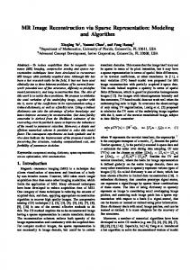
Figure 1: Equivalent representations of the same waveform in (a): time domain and (b): correlation domain. where, dc is the channel length between the transmitter and the receiver, vs is the speed of the ranging signal in the medium, tp is the time-period of the transmitted signal p(t), and tr is the approximate reverberation time within which the echoes from the transmitted pulse should have fallen below an acceptable level before the next pulse is emitted. The corresponding discrete-time signal of p(t) and x(t) obtained at a sampling rate (hertz/samples per second) of Fs is given as: p[np ] = p[tp Fs ] and x[na ] = x[ta Fs ] 0 ≤ np , na ≤ ∞. Therfore, p(t) and x(t) can be represented as vectors p ∈ Rnp and x ∈ Rna . Fig. 1(a) shows a received signal trace recorded for a duration of 0.1 s sampled at 48 kHz, and its cross-correlation with the reference copy (a linear chirp of [1-20] kHz/0.01 s) is depicted in Fig. 1(b). Although, obtaining the range using Eq. 8 and Eq. 9 is efficient, it requires the total knowledge (or samples na ) of the received signal x. Therefore, our objective (problem statement) is: Given significantly fewer (known) observations of x, obtain the cross-correlation result (unknown) s and estimate the range by finding the position of the first tallest peak.

2.2.1

Design of Dictionary for Cross-Correlation

The problem can be casted into the framework of sparse approximation (for solving underdetermined systems) by designing a dictionary that sparsely describes the received signal. With respect to ranging, the dictionary should also (precisely) capture the characteristic of the ranging pulse

Problem Statement

The cross-correlation method of detection and range estimation finds the position of the first tallest peak, which signifies the time-delay of the received signal x(t) with respect to its transmitted replica p(t). Cross-correlation of p(t) and x(t) is a sequence s(l) defined as: ∞ X s(l) = p(t + l)x(t) l = 0, ±1, ±2, ... (8)

Cross-Correlation / Correlation Domain

0.2

Normalized Magnitude

2.2

Time Domain 0.4

Amplitude

the sparse s accurately, even if the sensing matrix Ψ does not satisfy RIP. In fact, the use of `1 -minimization to find sparse solutions has a rich history. It was first proposed by Logan [20], and later developed in [13, 21–26]. Here, we use `1 -minimization to solve the cross-correlation problem via sparse representation. Dimensionality Reduction by Random Linear Projections: As shown in [27] by the Johnson-Lindenstrauss Lemma, the `2 distance is preserved in the projection domain with high probability by random projections. In other words, all the useful information is preserved in the projection domain. Hence, `1 -minimization can still be used to recover the sparse s from the projected measurements with an overwhelming probability, even though, its dimension is significantly reduced. More precisely, this projection from high to low dimensional space can be obtained by using a random sensing matrix Φ ∈ Rm×n as:

Signal Representation in Different Domains 1 FFT DCT Correlation

0.5

Threshold

0.1 0 0

2000

4000 6000 Samples

8000

10000

Figure 2: The signal has a more sparse representation in the correlation domain than the FFT and DCT domains by an order of more than 2.

that includes channel multipaths and low-noise signals, and facilitates the derivation of the range estimate from the reconstruction process without recovering the signal entirely. We propose a new dictionary Ψ for ranging: correlation domain that satisfies all of the three requirements. 1. Sparsity: It can be explained by Fig. 1(b), where only 4 samples (corresponding to the direct and other multipaths) out of the total 4800 samples are of significance as their peak heights are the most dominant among others that take on zero or negligible values resulting in a sparse depiction of the received waveform. 2. Preservation of channel profile: The index of the nonzero elements (i.e., correlation peak positions) define the multipath characteristic, and their coefficient values (i.e., correlation peak heights) provide an estimate of their contribution. 3. Implicit TOA: The (correlation) coefficient vector obtained from the recovery algorithm provides the measure of time-delay without further processing. In contrast, other popular dictionaries such as the FFT and DCT do not provide as good a sparse approximation as the proposed correlation domain, and also, do not satisfy the remaining two requirements (important for ranging). Fig. 2 compares their sparsity levels (for an indoor high multipath channel) by sorting the samples by their magnitudes. The fastest decay characteristic (or the smallest k) is observed in the correlation domain, and so, offers the most sparse representation; which means that the most accurate approximations (or range estimates) can be obtained in this dictionary using the smallest number of measurements m (Eq. 7).

2.2.2

Compression and Recovery

Compression: The dimensions of x ∈ Rna are significantly reduced at the receiver by multiplying it with a random sensing matrix Φ ∈ Rm×na resulting in the measurement vector y ∈ Rm (m  na ) as: y = Φx. m is related to na by the compression factor α given as: m = α na where α ∈ [0, 1]. For example, α = 0.10 means that the information in x has been compressed by 90%. Φ is a binary sensing matrix with its entries identically and independently (i.i.d.) sampled from a symmetric Bernoulli distribution. 1 ¯ ¯ i i.i.d. Pr(Φ ¯ i,j = ±1) = 0.5 where Φ Φ= √ Φ m

(10)

(`1r ) : ˆs1 = arg min ksk`1 s.t: ||ΦΨs − y||2 ≤ 

(12)

(`1r ) is a stable version of `1 -minimization. It is known as Lasso2 in statistical literature, and regularizes highly undetermined linear systems when the desired solution is sparse. The correlation domain coefficients ˆs1 are related to the various propagation (direct and reflected) paths, where the index of the first tallest correlation coefficient peak is the estimate of the pulse arrival time of the direct path, and thus, provides the range.

3

Empirical Study and Analysis

In this section, we validate the proposed detection method on a proof-of-concept (POC) acoustic ranging system (Fig. 3), explore performance improvements, and present results of various characterization studies. 1

Direct cross-correlation in the projection domain (using y) did not produce desirable ranging results because y consists of random projections. 2 The minimizer of kx − Ψsk22 + λkxk1 is defined as the Lasso solution; where λ can be referred as the inverse of the Lagrange multiplier associated with a constraint kx − Ψsk22 ≤ . For every λ, there is an  such that the two problems have the same solution.

OUTPUT CHANNEL

R

L Stereo Audio Card L INPUT CHANNEL

R

Figure 3: POC System Architecture.

Acoustic Pulse

(11)

Case-2 (ta >tp ) : The size of x is greater than p, and so, the system is balanced by right zero-padding (na − np ) entries to p. Since, x can be represented sparsely as s in the dictionary Ψ and x (the received signal) is known, the desired sparse solution s can be recovered by solving the `1 -minimization problem Eq. 5 (with dimensions of x reduced significantly via Eq. 61 ) that results in the following reduced `1 - minimization problem for a given tolerance :

Electronic Pulse

Binary ensembles have a shorter memory representation than Gaussian ensembles, and also, alleviate operational complexity; hence, are economical for sensor platforms. The receiver transfers m samples of y to the base-station (BS) for postprocessing. Recovery: The BS requires a-priori knowledge of the seed that generates Φ and the dictionary Ψ. Ψ is the positive and negative time shifted Toeplitz matrix of the transmitted signal vector p. Case-1 (ta = tp ) : Vectors p and x are of equal dimensions with na samples. The elements of Ψ ∈ Rna ×(2na −1) are given as:  [zeros(na − i) p(1 : i)]T 1 ≤ i ≤ na    T Ψ(:, i) = [p(i + 1 − na : na ) zeros(i − na )]    (na + 1) ≤ i ≤ (2na − 1)

where Ψ(:, i) denotes the ith column, [ ] denotes a vector of length na , zeros(i) denotes a zero vector of length i, ·T denotes the transpose of a vector (matrix), and p(i : j) denotes a vector of elements with indices from i to j of the input sample set p. For example, if p = [x1 x2 ... xn−1 xn ], then:   0 0 . . 0 x1  0 0 . . x1 x2        . . . . . . T Ψ = x2 . . xn−1 xn    x1  . . . . . .  xn−1 xn . . 0 0   xn 0 . . 0 0

3.1

POC System Architecture

3.2

Hardware: The transmitting front-end consisted of a ribbon (speaker) transducer driven by an external wideband (power) amplifier with a tunable gain controller [5x-20x]. The receiving front-end consisted of a custom designed receiver mounted with Knowles microphone (SPM0404UD5) attached to a preamplifier PCB. Ranging: The synchronization and ranging signals were generated, captured and analyzed using a laptop. A linear chirp [01-20] kHz/0.01 s was generated and directed into two separate streams: left input channel of the ADC of the audio card and wideband amplifier. The electronic chirp (directed into the ADC) is equivalent to an RF pulse and marks the time of transmission of the acoustic chirp when its amplified version is emitted by the speaker. The acoustic chirp is detected by the receiver and directed into the right input channel of the ADC. The final acoustic signal is considered from the TOA of the electronic chirp. The processing stage replicates the working of the receiver and BS, wherein the acquired samples are first compressed and subsequently recovered to estimate the range. In the experimental setup, the transmitter and the receiver were placed 1.5 m apart. The ranging process was performed with the receiver configured to record for 0.03 s - just long enough to capture the ranging signal along with its multipaths. The audio card was configured to sample at 48 kHz; hence, the transmitted signal p and the acquired trace x consisted of 480 and 1440 samples respectively. Using α = 0.30, x was compressed to obtain the measurement vector y of 432 samples followed by its recovery to obtain s (Section 2.2.2). Its accuracy was validated against standard cross-correlation (Eq. 8). Fig. 4(a) and Fig. 4(b) show the respective results, where we observe that both the methods obtain exactly the same estimate for the position of the first tallest peak at a negative lag of 220 samples along with the remaining multipath profile. The generation of the domain coefficients and cross-correlation peaks are in the negative lag part since we have reversed the order of operation, wherein the reference signal was operated with the acquired signal. Although, the remaining reconstructed peaks do not follow the same height-to-position relationship (observe the position of peak2 & 3 in Fig. 4(a)) as is expected from the corresponding cross-correlation result (Fig. 4(b)), they are not important parameters for distance estimation. This study validates our proposed algorithm for detection and ranging.

Correlation: 1440 Samples with 480 Samples 30 Lag: -ve Lag: +ve 1 25

Reconstruction: 432 Samples with 480 Samples 0.1 Lag: -ve 1 Lag: +ve

Magnitude

Magnitude

0.08 0.06 3 2

0.04

4

0.02 0 0

A vital point of difference between existing techniques and the proposed method is the functionality algorithm on the receiver: cross-correlation vs. compression. Conventional systems execute the cross-correlation algorithm on the receiver, whose implementation has a running time of O(n2 ) in the time domain (TD-CC) and O(n log n) in the frequency domain (FD-CC). However, due to no hardware divide or floating point support on WSN nodes, additional signal processing platforms have to be added. We propose an alternate data compression functionality that has a similar time complexity (mn ≈ O(n log n)), but a much smaller space complexity (competent with the mote constraints). In order to compare their performance on the POC system, we performed the same ranging process but configured the receiver to record for 0.1 s (i.e., 4800 acquired samples). Table 1 shows the individual running time of the TD-CC, FD-CC and compression for different compression factors α. We note that FD-CC is ≈ 30 times faster than TD-CC as expected from their asymptotic results. However, the compression time (shown as ‘Compression 1-Buf’) varies for different α, and is slower than FD-CC for all except α = 0.05. We overcome this drawback by using the simple idea of buffer-by-buffer compression rather than one-step compression. This method divides the acquired signal vector x of length na across b buffers of equal sizes, compresses the information in each buffer, and finally, assembles the measure˜ is ments in their correct order. The signal in each buffer x of length n ˜ , where n ˜ = na /b. The random sensing matrix Φ for compressing the data in each buffer is of size [m ˜ ×n ˜ ], where m ˜ = αn ˜ = α (na /b) = m/b. The resultant mea˜ (for each buffer) is of length of m. surement vector y ˜ The number of iterations required to process each buffer is (m˜ ˜ n). Therefore, the compression time for b buffers take (bm˜ ˜ n) = (mna /b) iterations. This improvement can be identified in Table 1 (shown as ‘Compression 10-Buf’), where we divide the 4800 samples across 10 buffers and record their individual compression time for different α. The results show a worst-case to best-case improvement of 6× to 60× over FD-CC. A greater improvement is expected on sensor platforms (shown in Section 5) than PC as they do not support floating point operation.

3.3

960

1440 1920 Samples

(a)

2400 2800

Signal Detection and Post-processing

The process of detection is not without errors as the reconstructed coefficients s may have been wrongly approximated due to measurement noise that contributes to higher coefficient values at incorrect locations. To overcome these inaccuracies, we use the same principle of buffer-by-buffer reconstruction at the BS as well, which not only provides an additional clue for correct detection, but also, serves as a guideline to choose the buffer count b.

20 15

3

10

2

4

Table 1: Performance Analysis: PC

5 480

Performance Analysis and Improvement

0 0

480

960

1440 1920 Samples

2400

2880

(b)

Figure 4: Correlation Domain Coefficients and standard Cross-Correlation obtain the same result for the position of the LOS peak.

α 0.05 0.10 0.30 0.50

TD-CC (sec) 0.1932 0.1932 0.1932 0.1932

FD-CC (sec) 0.0062 0.0062 0.0062 0.0062

Compression 1-Buf (sec)

Compression 10-Buf (sec)

0.0042 0.0077 0.0218 0.0361

0.0001 0.0003 0.0006 0.0010

Reconstruction in Buffers [Buf-1] 144 Samples with 480 Samples

Reconstruction in Buffers [Buf-2] 144 Samples with 480 Samples

0.1 Lag: +ve

Lag: -ve 1 2

0.08 Magnitude

Magnitude

0.08

0.1

0.06 0.04

1Lag: +ve

Lag: -ve 2

0.06

r = ((˜ nbi−1 + ˆ l)/Fs ) × vs

3

0 0

0.02 200

400 600 Samples

800

0 0

960

200

(a) Lag: -ve

25 Magnitude

Magnitude

960

1 2

10 5

Lag: +ve

Lag: -ve

20

1

15

2

10

4

3

5 200

400 600 Samples

(c)

800

960

0 0

200

400 600 Samples

800

where bi−1 is the buffer count before the detection buffer, ˆ l is the lag (in samples) of the ranging peak in the detection buffer, and vs is the temperature compensated speed of sound in air.

3.4

30 Lag: +ve

20

0 0

800

Correlation in Buffers [Buf-2] 480 Samples with 480 Samples

30

15

400 600 Sampes

(b)

Correlation in Buffers: [Buf-1] 480 samples with 480 samples 25

(13)

0.04 4

0.02

If ˜b = 1 (i.e., only a single buffer has a valid peak), then the peak identified in phase-1 qualifies as the ranging peak. The estimated range r is obtained as:

1,000

(d)

Figure 5: Buffer-by-Buffer Processing: Reconstruction of Correlation Coefficients and CrossCorrelation obtain the same result for the position of the LOS peak, and the tallest peak in each buffer. The number of buffers b is chosen such that the number of samples in each buffer is the same as the sample count of the reference signal p, i.e., n ˜ = tp Fs . For example, if p contains 100 samples and x consists of 1000 samples, then b is 10. There are two benefits in making this choice. First, it restricts the direct path signal (in the total acquired trace) to be spread across a maximum of 2 buffers, and so, guarantees that the magnitude of the corresponding recovered coefficient would always remain at least 50% above its original estimate. Increasing b beyond 2 buffers decreases the individual peak heights to smaller magnitudes that poses a difficult detection task to differentiate them from the noisefloor. Second, it provides easy processing at the BS, where the operation of right zero-padding p to make its dimensions equal to x is substituted by fragmenting x into b buffers to match the size of p (Section 2.2.2). The reconstruction process is performed on all b buffers, which is followed by the signal detection and range estimation algorithm. Phase-1: It identifies the various correlation domain coefficient peaks and selects the first tallest peak in each of the b buffers that is atleast 6 standard deviations above the mean. The detection is considered to have failed for those buffers where no point qualifies as a peak. This reduces the validation space for phase-2 to ˜b (≤ b) buffers. Phase-2: If there are valid peaks in more than one buffer (i.e., ˜b > 1), then the tallest peak (across all ˜b buffers) among them is selected as the ranging peak. The detection is correct, if this peak in buffer bi has a lag that is: • Positive: ⇒ The peak in the previous buffer bi−1 must have a negative lag. • Negative: ⇒ The peak in the next buffer bi+1 must have a positive lag. This relationship is a result of the manner in which the signal gets aligned in different buffers and its equivalent representation in the correlation domain/cross-correlation (Fig. 5).

Characterization of Compression Factor

One of the key decisions is to choose the optimal compression factor α thats achieves the best accuracy with the least measurements (or projections) m, where a smaller m leads to lower storage and transmission cost. α depends on the sparsity k (Eq. 7) of the received signal in the correlation domain, which in turn depends on the received SNR that varies with transmission power and ranging distance. In this subsection, we empirically study the relationship between SNR and α. The study was conducted in the following environments. Case-A - Outdoor, Very low multipath: A less frequently used urban walkway, and the weather being sunny with occasional mild breeze. Case-B - Indoor, Low multipath: A quiet lecture theatre ([25 × 15 × 10] m) with a spacious podium at one end of the large room. Case-C - Indoor, High multipath: A quiet meeting room ([7 × 6 × 6] m) with a big wooden table in the center and other office furnitures. The transmitter and the receiver were fixed at a constant separation distance of 5 m. The transmit power was varied such that the received SNR were recorded within the limits: [0-5) dB, [5-10) dB, [10-20) dB, [20-30) dB. For reasons that will be explained in the next subsection, we slightly modified the peak selection criteria of the detection algorithm to choose the tallest peak if there was no valid peak (6 standard deviation above the mean). 100 observations were collected for every experiment. We show the relative mean error and its deviation with respect to the (best-case) standard crosscorrelation in all the results in this subsection. Fig. 6(a), Fig. 6(b) and Fig. 6(c) shows the dependence of α-compression and its recovery accuracy on the SNR of the ranging signal. Across all figures, we observe that applying a higher α on a lower SNR signal results in an increase in estimation error. Fig. 6(a) for Case-A presents the most clear characterization by negating the effect of channel multipaths (though introducing an increased background noise level), where observations with a high SNR of [20-30) dB provide reliable range estimates by using only 15% projections while those having low SNR of [0-5) dB show confident result only with α = 0.30 (i.e., using more projections). Fig. 6(b) and Fig. 6(c) show the results for Case-B and CaseC. Due to a less dominant multipath profile and background noise in Case-B, the accuracy levels show high confidence for α ≥ 0.20. The situation is challenging in Case-C (due to high multipath), and so, the errors are as large as 1 m with α = 0.05, but attain stability after α = 0.25. The cumulative probability results suggest that there is a 95% probability of incurring an additional error of < 1.5 cm in indoors and < 3 cm in outdoors with α = 0.30 with respect to its standard cross-correlation estimate. Using α > 0.30 does not improve the accuracy significantly considering the

140

140

[20-30) dB [10-20) dB [05-10) dB [00-05) dB

100 80 60 40 20

100 80 60 40 20

0 0

Correlation Domain Indoor: Meeting Room

[20-30) dB [10-20) dB [05-10) dB [00-05) dB

120 Mean Error (cm)

120 Mean Error (cm)

Correlation Domain Indoor: Lecture Theatre 140

100 80 60 40 20

0 0.05

0.10 0.15 0.20 0.25 Compression Factor

0.30

0

0

(a) Case-A: Very-low Multipath

[20-30) dB [10-20) dB [05-10) dB [00-05) dB

120 Mean Error (cm)

Correlation Domain Outdoor Walkway

0.05

0.10 0.15 0.20 0.25 Compression Factor

0.30

0

(b) Case-B: Low Multipath

0.05

0.10 0.15 0.20 0.25 Compression Factor

0.30

(c) Case-C: High Multipath

Figure 6: Characterization of Compression Factor α with SNR.

2

10

0

10

-2

[00-05)

2

10

0

10

-2

[05-10) [10-20) SNR (dB)

10

[20-30)

(a)Improvement: Order of mag. 1

[00-05)

Buffer-by-Buffer vs. Single Buffer Detection Method Indoor: Meeting Room 4 10 Buf-by-Buf Single Buf

Log (Mean Error)

10

Buffer-by-Buffer vs. Single Buffer Detection Method Indoor: Lecture Theatre 4 10 Buf-by-Buf Single Buf

Log (Mean Error)

Log (Mean Error)

Buffer-by-Buffer vs. Single Buffer Detection Method Outdoor Walkway 4 10 Buf-by-Buf Single Buf

2

10

0

10

-2

[05-10) [10-20) SNR (dB)

[20-30)

(b)Improvement: Order of mag. 1.5

10

[00-05)

[05-10) [10-20) SNR (dB)

[20-30)

(c)Improvement: Order of mag. 4

Figure 7: For a compression factor of 0.30, the Buffer-by-Buffer detection shows an order of magnitude 1-4 improvement over Single Buffer detection method. additional overheads. Fig. 6 also shows that for applications that require lower accuracy (e.g., 100 cm), α as less as 0.05 is sufficient. We also performed ranging experiments with changes in distance over 1-10 m. Although, smaller values of α (i.e., lesser projections) were good for high SNR levels, the results with α = 0.30 were optimal, even in the worst case to obtain higher accuracy (< 2 cm). Fig. 7 compares the detection accuracy between our proposed buffer-by-buffer method versus processing all the samples in a single buffer. From reasons explained in Section 3.3, the results show at least 1 order of magnitude improvement. The sparse representation in the proposed correlation domain shows significantly better accuracy of an order of magnitude 2 (Fig. 8) compared to the DCT domain (for α=0.30) due to the most sparse depiction of the ranging signal (Fig. 2). For DCT domain processing, the recovered coefficients ˆs1 were multiplied with the DCT basis Ψ (Eq. 1) to obtain an ˆ 1 , and then cross-correlated estimate of the received signal x with the reference signal p. Another simple (but deterministic) method of reducing the sample count is to downsample x by a factor Fd resultˆ . We verify its detection accuracy in the correlaing in y tion domain by using two different algorithms: (a) standard cross-correlation and (b) sparse approximation problem formulated as: 0

ˆ ||2 ≤  (`1r ) : ˆsd1 = min ksk`1 subject to:||Ψ s − y

(14)

The comparison results in Fig. 8 show that neither of these two methods based on downsampling provide better estimates than the proposed method of `1 -minimization in the correlation domain where the improvement is of an order of magnitude 2 across all experimental environments. This improvement is the result of information embedding in random ensembles that preserves the `2 -norm (or energy) of its respective higher dimension representation, as opposed to deterministically choosing samples and discarding information (i.e., frequency components) by downsampling. It supports the theoretical result that there is an overwhelming probability of correct recovery via `1 -minimization for dimensionality reduction by random linear projection (Section 2.1).

3.5

Adaptive α-Estimation

The design of an adaptive mechanism for α requires estimating the received SNR. We propose two different approaches: first, with a BS feedback to receiver, and second, on the receiver itself. For the BS-feedback mechanism, we utilize empirical information from the peak detection algorithm. In Section 3.3, we considered the scenarios where the valid buffer count ˜b ≥ 1. If a valid peak (i.e., at least 6 standard deviations above the mean) is not detected in any buffer (i.e., ˜b = 0), then the detection is considered to have failed. This implies that the recovered coefficients are noisy due to a nonoptimal α for the respective measurements (characterized by its SNR). It was precisely the reason for modifying the peak

10

6

10

4

10

2

10

0

10

-2

Corr Domain + CP + L1-min DCT Domain + CP + L1-min DS + Std. Cross-Correlation Corr Domain + DS + L1-min

[00-05)

10

Corr Domain + CP + L1-min DCT Domain + CP + L1-min DS + Std. Cross-Correlation Corr Domain + DS + L1-min

6

10

4

10

2

10

0

10

-2

[05-10) [10-20) SNR (dB)

[20-30)

(a)Improvement: Order of mag. 1-4

10

[00-05)

Domain and Algorithm Comparison Indoor: Meeting Room

8

10

Corr Domain + CP + L1-min DCT Domain + CP + L1-min DS + Std. Cross-Correlation Corr Domain + DS + L1-min

6

Log (Mean Error)

10

Domain and Algorithm Comparison Indoor: Lecture Theatre

8

Log (Mean Error)

Log (Mean Error)

Domain and Algorithm Comparison Outdoor Walkway

8

10

4

10

2

10

0

10

-2

[05-10) [10-20) SNR (dB)

[20-30)

(b)Improvement: Order of mag. 2-4

10

[00-05)

[05-10) [10-20) SNR (dB)

[20-30)

(c)Improvement: Order of mag. 4

Figure 8: For a compression(CP)/downsampling(DS) factor of 0.30, the proposed sparse approximation method based on compression with `1 -min in the correlation domain shows an order of magnitude 1-4 higher detection accuracy compared to: (i) compression with `1 -min in the DCT domain (ii) downsampling with cross-correlation (iii) downsampling with `1 -min in the correlation domain. selection criteria in the previous subsection, where we observed large errors in peak positions for magnitudes below the specified threshold. The BS-feedback algorithm starts with the initial knowledge of whether a valid peak was determined with α = 0.30. If the detection succeeds, then α is decremented by a step size of 0.05 and compressed. This process is iterated until the detection fails, in which case, the previous α values is selected. On the other hand, if no valid peaks were encountered for the starting case, α is incremented in steps of 0.05 and the entire process is repeated until the detection succeeds. A major drawback of the feedback approach is the additional measurements (that translate to transmission overhead), and its associated delay and power usage for deriving α. Therefore, we introduce this functionality on the receiver by a simple power estimation algorithm. The ratio ρ of the peak signal amplitude to the average of the absolute values in the sampled signal is calculated, and a corresponding α is selected according to the following empirically chosen criteria. α = {{0.05 : ρ > 30}, {0.10 : 20 < ρ ≤ 30}, {0.10 : 20 < ρ ≤ 30}, {0.20 : 15 < ρ ≤ 20}, {0.30 : 10 < ρ ≤ 15}, {0.50 : 05 < ρ ≤ 10}, {1.00 : ρ ≤ 05}}. For our analysis, we randomly selected 1000 measurements pertaining to different SNR levels in the indoor lecture theatre (Case-B). The respective α was estimated using the above two methods and their performance was compared against our empirically selected threshold value of α = 0.30. Table 2 reports their performance trade-off where the BSfeedback obtains high accuracy but requires 2 times more measurements, while the receiver estimation approach takes fewer measurements and obtains only a 5% worse accuracy.

Table 2: Projections vs. Accuracy: A positive value indicates higher projections or reconstruction error compared to the threshold α = 0.30 Scenario BS-Feedback Receiver

Projections (%) 101.16 -17.55

Accuracy (%) -1.75 5.26

4

End-to-End System Architecture

In this section, we present the implementation of an endto-end acoustic ranging system. Its design was driven by the specific goal of fast data acquisition and compression on the receiver node, which could be achieved by performing all operations on the mote’s RAM without involving its external flash that would introduce additional latency. Therefore, all design decisions were guided towards maximum RAM utilization.

4.1

System Design: Hardware & Software

The system comprised of the TmoteInvent (as listener), our designed sensor mote (as beacon) and a network interface to the base-station (Fig. 9). Transmitter: The beacon node (Fig. 10) comprised of our WSN platform along with a custom designed audio daughter board that included four TI TLV320AIC3254 audio codecs, each providing two audio I/O channels and a connector to hold the Bluetechnix CM-BF537E digital signal processor module. The transmitting front-end of the beacon mote consisted of a power amplifier driving a tweeter (speaker) transducer (VIFA 3/4” tweeter module MICRO). The tweeter (size: [2 × 2 × 1] cm) had a fairly uniform and high frequency response of ≈ 22 dB above the noise-floor between 1-10kHz. Receiver: TmoteInvent [29] was used as the listener node, due to its low-cost and low-power (100 times more power efficient than the DSP on the transmitter) features that are expected from a WSN platform. The receiving front-end consisted of an omni-directional electret microphone (Panasonic WM-61B) attached to an Analog Devices SSM2167 preamplifier. It allows omni-directional acquisition in the range 20 Hz - 10 kHz, and has a near-flat frequency response between 3-7 kHz that is 10 dB above the noise floor. Highrate audio data collection was achieved using the DMA controller packaged with the MSP430 MCU. The driver for the acoustic daughter board performs DMA acquisition to coordinate the transfer of samples from the ADC conversion registers to sequential words in RAM, and generates an interrupt on filling the assigned RAM buffer with data. Delay between fetching a new buffer for the DMA to fill was minimized by prefetching an additional spare buffer and making it available at the instant it was requested. However, the MSP430 DMA causes truncation of the 12 bits ADC data

SOFTWARE

RF TCP IP/ Directory Poll

Serial

RF

Packet Listener

Acoustic Packet Simulator Transmitter

Receiver

Base Node

Reconstruction & Localization Algorithm

Display/ Database

Base Station

Figure 9: System Architecture of the End-to-End Acoustic Ranging System.

Audio Codec

Power Amplifier

SPI 2.4 GHz Radio

Speaker

Blackfin DSP Serial Fleck

Figure 10: Transmitter Node: CSIRO Audio Mote.

to 8 bits rather than to two bytes, and so, results in a data resolution loss of 4 bits.

4.2

Ranging and Detection Methodology

The system uses the time-difference-of-arrival (TDOA) of RF and acoustic signals to measure the beacon-to-listener distance. The beacon initiates the ranging process by periodically transmitting a RF signal followed by a acoustic pulse after a fixed time interval. The fast propagating RF pulse reaches the listener almost instantaneously and synchronizes the clocks on both the devices, following which, the TDOA is measured after the arrival of the acoustic pulse. The ranging signal was a linear chirp of [3-7] kHz/0.01 ms and was transmitted at an acoustic pressure level of 70 dB. The DAC on the audio codec of the beacon node was programmed to sample at 48 kHz, while the ADC on the receiver Tmote was configured to acquire at 15 kHz. If the time taken for sound to travel a maximum range dc at a speed vs is at most dvsc , and if the transmitted chirp length is tp , then the signal must reach the receiver within [ dvsc + tp ]. For tp = 0.01 s and dc ≈ 10m, the recording of the signal must be completed by 0.03 s. We include an additional 0.01 s to compensate for reverberation time (tc ), and setup the recording time to 0.04 s (Eq. 9). Following the buffer-by-buffer compression method, the signal was spread ¯ was stored in the across 5 buffers. A measurement matrix Φ RAM that contained i.i.d. entries sampled from a symmetric Bernoulli distribution (Eq. 10). We postponed the multiplication √ operation on the matrix entities with the constant (1/ m) until the recovery stage at the BS. The listener acquires the audio samples, compresses and stores these measurements in the RAM over a period of 5 iterations, and then, transfers them to the BS. These measurements are again divided into their respective buffers and reconstructed to obtain the coefficients. The detection process is the same as explained in Section 3.3, however we

made two minor modifications. First, due to a higher receiver noise floor, we set the criteria for selecting the first tallest peak to 3 (instead of 6) standard deviations above the mean. Second, as each sample corresponds to 2.2 cm of distance (at a sampling rate of 15 kHz), we used a simple parabolic interpolation method to obtain finer resolution. This additional step identifies the position of the first neighboring peak on the left and right of the selected ranging peak, finds the parabola that passes through these points, and calculates the time coordinate of the maximum of this parabola that estimates the range.

5

Evaluation: Experimental and Performance

Ranging: The ranging experiments were performed in the same three environments as mentioned in Section 3.4: (a) Case-A: outdoor walkway, (b) Case-B: lecture theatre, and (c) Case-C: meeting room. In all the setups, the listener node was fixed while the beacon node was moved along the direct LOS in a controlled manner. The correct ground truth was established using a measuring tape and markers. The evaluation results are shown in Fig. 11, where we plot the absolute mean error and standard deviation for both standard and `1 -min cross-correlation with respect to the ground truth. The best results were obtained in Case-B (Fig. 11(b)) where the mean error for `1 -min was recorded as ≈ 9 cm at the maximum measured distance of 10 with a maximum deviation of ≈ 11 cm with respect to ground truth. Its maximum deviation from standard cross-correlation was ≈ 2 cm. Due to the decrease in the sparsity levels with lower SNR, the measurements from [6 − 10] m were compressed with a higher α of 0.35. Fig. 11 (a) and Fig. 11 (c) show the results for CaseA and Case-C, where the mean errors and deviations are significantly higher than Case-B (even at short range [1 − 5] m). The sparsity of the received signal was affected by the high background noise and multipath in the respective environments, and hence, resulted in incorrectly approximated range values. Also, we observe a maximum error difference of ≈ 5-6 cm between the two algorithms. In Case-A, α = 0.40 was used for compressing data after 5 m of measurement distance. The audio recordings after 8 m were highly noisy and required an even higher α value for compression. However, due to non-availability of RAM memory space for storing the additional entries of the new measurement ma¯ range estimates beyond 8 m could not be processed. trix Φ, There was no scope for adaptive α-estimation (Section 3.5) as the empirically chosen values were the absolute minimum required for reliable recovery. Localization: In these experiments, 5 listener nodes were placed at fixed (known) locations in a [4 × 5] m area of the

30

Standard Cross-Correlation L1-min Cross-Correlation

Abs. Mean Error (cm)

Abs. Mean Error (cm)

30

Range Measurments Indoor: Lecture Theatre

20 10 0 -10 0

1

2

3 4 5 6 7 True Distance (m)

8

Standard Cross-Correlation L1-min Cross-Correlation

20 10 0 -10 0

9

Range Measurments Indoor: Meeting Room

(a): Case-A: Very-low Multipath α = {0.30 (1-5 m), 0.40 (6-8 m)}

1

2

3 4 5 6 7 8 True Distance (m)

9 10 11

(b): Case-B: Low Multipath α = {0.30 (1-5 m), 0.35 (6-10 m)}

30 Abs. Mean Error (cm)

Range Measurements Outdoor Walkway

Standard Cross-Correlation L1-min Cross-Correlation

20 10 0 -10 0

1

2 3 4 True Distance (m)

5

6

(c): Case-C: High Multipath α = {0.30}

Width (m)

Figure 11: End-to-End Acoustic Ranging System: Ranging results.

Node Placement and Localization Results Indoor: Lecture Theatre 0 LISTENER BEACON 1 STD-XCORR CS-XCORR 2 3 4 -1

0

1

2 3 Length (m)

4

5

6

Figure 12: Localization result.

indoor lecture theatre (Case-B) to obtain the (unknown) location coordinates of the beacon node. The speaker had a fairly uniform signal strength within the directionality cone of ± 45o (with a 2 dB decrease from 0o − 45o ), therefore, all the 5 listeners were confined within this perimeter with their microphones facing the speaker. The beacon initiated the ranging process and the corresponding acoustic chirp was recorded by the 5 listeners. A simple time division multiple access (TDMA) approach was followed for orderly data transfer wherein each listener transferred the compressed data in a preset time slot. The distances between the beacon and the receivers were estimated at the BS, which was followed by the linear least square localization algorithm to calculate the 2D location of the beacon node. Fig. 12 shows the node placements, where the listener and beacon node(s) have been depicted as circle and square respectively along with the estimated beacon location using the two methods. The standard and `1 -min cross-correlation show similar results with a mean localization error of 18 cm and 17 cm with a deviation of 6 cm and 7 cm respectively. As the localization error is upper bounded by its ranging errors, we expect similar relative performance in Case-A and Case-C that show a maximum ranging error difference of 5 cm.

Table 3: Performance Analysis: TmoteInvent Operation

Time (s)

Energy (mJ)

Audio Acquisition

00.0665

0020.50

Compression Radio Transfer (Compressed Data)

00.0060 00.0580

0001.85 0017.88

Cross-correlation (Time-domain)

15.6250

4816.00

Energy Consumption: Table 3 reports the time and energy consumed for each operational step on the listener node. The cumulative time spent in compression and radio transfer is ≈ 0.0640 s, which is more than 100 times faster than performing time-domain cross-correlation on the node itself. Its equivalent frequency-domain cross-correlation requires 2*FFT and IFFT operation steps. When optimized for speed, a FFT over 512 sample window of an 8 kHz signal takes 0.5 s execution time on TelosB [30], and so, for our case of 750 samples would take ≈ 2.2 s, which is still 34 times slower. With respect to compression performance, the popular LZ77-based algorithm ‘gzip’ achieves slightly better compressibility of α = 0.27 (Table 4). However, due to its lossless nature of compression, it is not robust to information loss (packet drops) that are common in low-power sensor networks. In contrast, the performance degradation by our approach is less severe and has the same effect as compressing with a smaller α (Fig. 6). A similar, but energy efficient algorithm proposed by Sadler et al. [31]: S-LZW reports an execution time of approximately 0.05 s for 528 bytes of data, and therefore, its equivalent compressing cost

Table 4: Compression Factor (α) for LZ77-based Compression Algorithm ‘gzip’: Dataset collected by the POC System (Section 3.4). Scenario Case-A: Very-low Multipath Case-B: Low Multipath Case-C: High Multipath

Mean α

Deviation α

0.27 0.27 0.28

0.005 0.005 0.009

for 750 bytes would be approximately 0.075 s (≈ 12 times slower than our technique). These statistics suggest that although compression by random ensembles is not the best compression method, it benefits of greater energy savings along with faster data processing is a good trade-off between compression and computation time, accuracy (in case of data loss), energy consumption. For example, if applications can tolerate 100 cm localization accuracy, the proposed method requires approximately 5% of measurements only (Fig. 6). Furthermore, in the event of packet loss, SLZW needs to either retransmit the entire compressed data segment, or employ expensive end-to-end reliable communication protocol. On the other hand, the performance of the proposed protocol degrades gracefully with packet losses as it can still recover the ranging information, but with larger errors (Fig. 6).

6

Related Work

We broadly categorize the related work based on the detection mechanism used in existing acoustic, ultrasound and RF localization systems in WSN. Non Cross-correlation: Active Bat [1], Cricket [2], Medusa [3] and SpiderBat [32] are ultrasound positioning systems. Range measurements are performed by calculating the TDOA between two synchronously sent RF and ultrasonic pulses at the receiver. The ranging pulse is a single frequency (40 kHz) sinusoidal and its arrival is detected by triggering an interrupt pin of the microcontroller when its leading edge exceeds a preset threshold. Due to the functional simplicity, low-power microcontrollers (Atmega/MSP430 series) used in these platforms are efficient in managing the on-board processing. Kusy et al. in [33] introduced radio inferferometry to design a low-cost RF-based positioning system on the Mica2 platform. This method measures the relative phase offsets of the interference field (created by two nodes transmitting RF pulses at slightly different frequencies) at different locations to obtain the position estimate of the transmitters. However, these techniques are not robust against multipath characteristics, and so, no results have been published for complex cluttered environments. Cross-correlation: The system proposed by Kushwaha et al. in [7], Hazas et al. in [6], AENSBox [8], BeepBeep [9] and TWEET [10] are existing acoustic broadband systems. Despite their difference in signal design, synchronization schemes and methods to improve the received SNR, they share a common detection mechanisms:cross-correlation. These systems have been reported to withstand considerable channel multipath and environmental noise, and so, benefit in providing reliable and precise distance estimates for long coverage range. However, the capability of these systems have been upgraded by using DSP/smart phones that typically consume higher power and resources. The theory of sparse representation [13] helps to efficiently embed information without much loss (which serves the purpose of storage and transmission) followed by its recovery from an underdetermined system. Although, we follow a similar approach as Wright et al. [28] in face recognition, the scope of our problem is completely different. We design a new dictionary, specifically, for cross-correlation based detection and ranging, as opposed to feature extraction for face classification.

Previous work by Whitehouse et al. in [11] and Sallai et at. in [12] on acoustic ranging in resource constrained sensor networks (using MICA platform) categorically state that the limited availability of RAM was the most serious constraint in their system implementation. The ranging results reported by [12] have an average error of 8.18 cm over a distance of 1-9 m by repeating the ranging signal 16 times, which results in significant runtime and energy overhead. Using cross-correlation via sparse representation, our acoustic ranging system was able to confront this problem, and also, was able to provide similar performance (mean error of < 10 cm over 1-10 m) with fewer samples.

7

Conclusion and Discussion

We presented a new information processing approach for range estimation: cross-correlation via sparse representation. We showed that exploiting sparsity is critical for highperformance signal processing operations of high-dimensional data such as cross-correlation. The sparsity of the underlying signal in our proposed correlation domain aids in the recovery mechanism to obtain reliable range estimates. The main idea was to use a Toeplitz matrix with the time-shifted reference signal as the dictionary that leads to sparser representation than processing in other domains such as DCT. We designed its theoretical framework and validated its working through empirical system tests and characterization studies. Considering the implementation simplicity in the acoustic domain, we developed an end-to-end acoustic ranging system using COTS sensor platforms to verify our hypothesis. The theoretical foundation of this work is based on sparse approximation, and not on compressive sensing that mandates strict adherence to the RIP condition. As explained in Section 2, RIP is only a sufficient but not a necessary condition for reconstruction accuracy; therefore, a stable solution is still recoverable by `1 -minimization. It is well understood that cross-correlation only solves a small part of the ranging problem, and therefore, our work is preliminary in the sense that we have not yet entirely evaluated the consequences of externalities. An intriguing question for future work is whether this framework can be useful with other challenges such as directional receivers, limited range and signal penetration, noisy background conditions and high-stress environments [34], scalability issues, etc. In addition, an indepth analysis of the properties of a Toeplitz matrix with respect to spare approximation and compressive sensing is also required for better design of sensing matrices. Furthermore, its ability to adapt to mobile conditions (for object tracking) needs to be evaluated, and executing it in a principled manner remains an important future direction. Our work in this paper is guided by the current hardware limitations of low-cost and low-power sensor platforms. We believe that the key observations and principles derived here will find their application in location sensing systems that have constrained hardware resources to handle the bulk of data processing.

8

Acknowledgment

We would like to thank the anonymous reviewers for their helpful comments; and Dr. Brano Kusy (CSIRO) and Dr. Philipp Sommer (CSIRO) for being internal reviewers. This work is supported by Sensors and Sensor Networks Transformational Capability Platform, CSIRO.

9

References [18]

[1] Andy Harter, Andy Hopper, Pete Steggles, Andy Ward, and Paul Webster. The anatomy of a context-aware application. In MobiCom, pages 59–68. ACM, 1999. [2] Nissanka Bodhi Priyantha. The Cricket Indoor Location System. PhD thesis, MIT, 2005. [3] Andreas Savvides, Chih-Chieh Han, and Mani B. Strivastava. Dynamic fine-grained localization in ad-hoc networks of sensors. In MobiCom, pages 66–179. ACM, 2001. [4] Evangelos Mazomenos, Dirk De Jager, Jeffrey S. Reeve, and Neil M. White. A two-way time of flight ranging scheme for wireless sensor networks. In EWSN. Springer-Verlag, 2011. [5] P. Misra, D. Ostry, and S. Jha. Improving the coverage range of ultrasound-based localization systems. In WCNC, pages 605–610. IEEE, 2011. [6] M. Hazas and A. Hopper. Broadband ultrasonic location systems for improved indoor positioning. IEEE TMC, 5(5):536–547, 2006. [7] M. Kushwaha, K. Molnar, J. Sallai, P. Volgyesi, M. Maroti, and A. Ledeczi. Sensor node localization using mobile acoustic beacons. In MASS, pages 9pp.–491. IEEE, 2005. [8] Lewis Girod, Martin Lukac, Vlad Trifa, and Deborah Estrin. The design and implementation of a self-calibrating distributed acoustic sensing platform. In SenSys, pages 71–84. ACM, 2006. [9] Peng Chunyi, Shen Guobin, Zhang Yongguang, Li Yanlin, and Tan Kun. Beepbeep: a high accuracy acoustic ranging system using cots mobile devices. In SenSys, pages 1–14. ACM, 2007. [10] P. Misra, D. Ostry, N. Kottege, and S. Jha. Tweet: An envelope detection based ultrasonic ranging system. In MSWiM, pages 409–416. ACM, 2011. [11] Kamin Whitehouse and David Culler. Calibration as parameter estimation in sensor networks. In WSNA. ACM, 2002. ´ [12] J´ anos Sallai, Gy¨ orgy Balogh, Mikl´ os Mar´ oti, Akos L´edeczi, and Branislav Kusy. Acoustic ranging in resource constrained sensor networks. In ICWN, page 04. CSREA Press, 2004. [13] David L. Donoho. For most large underdetermined systems of linear equations the minimal `1 -norm solution is also the sparsest solution. Communications on Pure and Applied Mathematics, 59(6):797–829, 2006. [14] P. Zhao and B. Yu. On model selection consistency of lasso. J. Machine Learning Research, 7:2541–2567, 2006. [15] R. Tibshirani. Regression shrinkage and selection via the lasso. J. Royal Statistical Soc. B, 58(1):267–288, 1996. [16] E. Amaldi and V. Kann. On the approximability of minimizing nonzero variables or unsatisfied relations in linear systems. Theoretical Computer Science, 209:237–260, 1998. [17] Edoardo Amaldi and Viggo Kann. On the approximability of minimizing nonzero variables or

[19] [20] [21]

[22]

[23]

[24]

[25]

[26]

[27]

[28]

[29] [30]

[31]

[32]

[33]

[34]

unsatisfied relations in linear systems. Theoretical Computer Science, 209(1-2):237 – 260, 1998. E. J. Candes and T. Tao. Near-optimal signal recovery from random projections: Universal encoding strategies? IEEE Trans. on Inf. Theory, 52(12):5406–5425, 2006. D.L. Donoho. Compressed sensing. IEEE Trans. on Inf. Theory, 52(4):1289–1306, april 2006. B. F. Logan. Properties of high-pass signals. Ph.D. Thesis, 1965. Donoho D. L. and B. F. Logan. Signal recovery and the large sieve. SIAM J. APPL. MATH., 52(2):577–591, 1992. S. S. Chen, D. L. Donoho, and M. A. Saunders. Atomic decomposition by basis pursuit. SIAM J. Scientific Computing, 20(1):33–61, 1999. D. L. Donoho and X. Huo. Uncertainty principles and ideal atomic decomposition. IEEE Trans. Inf. Theory, 47(7):2845–2862, 2001. R. Gribonval and M Nielsen. Sparse representations in unions of bases. IEEE Trans. Inf. Theory, 49(12):3320–3325, 2003. David L. Donoho and Michael Elad. Optimally sparse representation in general (nonorthogonal) dictionaries via `1 minimization. Proceedings of the National Academy of Sciences, 100(5):2197–2202, 2003. M. Elad and A.M. Bruckstein. A generalized uncertainty principle and sparse representation in pairs of bases. IEEE Trans. on Inf. Theory, 48(9):2558 – 2567, sep 2002. R. Baraniuk, M. Davenport, R. DeVore, and Wakin M. A simple proof of the restricted isometry property for random matrices. Constr Approx, 28:253–263, 2008. J. Wright, A. Y. Yang, A. Ganesh, S. S. Sastry, and Ma Yi. Robust face recognition via sparse representation. IEEE PAMI, 31(2):210–227, 2009. http://sentilla.com/files/pdf/eol/ tmote-invent-user-guide.pdf. Ben Greenstein, Christopher Mar, Alex Pesterev, Shahin Farshchi, Eddie Kohler, Jack Judy, and Deborah Estrin. Capturing high-frequency phenomena using a bandwidth-limited sensor network. In SenSys. ACM, 2006. 279-292. Christopher M. Sadler and Margaret Martonosi. Data compression algorithms for energy-constrained devices in delay tolerant networks. In SenSys, pages 265–278. ACM, 2006. G. Oberholzer, P. Sommer, and R. Wattenhofer. Spiderbat: Augmenting wireless sensor networks with distance and angle information. In IPSN, pages 211–222. ACM/IEEE, 2011. Kusy Branislav, Sallai Janos, Balogh Gyorgy, Ledeczi Akos, Protopopescu Vladimir, Tolliver Johnny, DeNap Frank, and Parang Morey. Radio interferometric tracking of mobile wireless nodes. In Mobisys. ACM, 2007. P. Misra, S. Kanhere, D. Ostry, and S. Jha. Safety assurance and rescue communication systems in high-stress environments: A a mining case study. IEEE Communication Magazine, 48(4):66–73, 2010.