Meng Xu, Xiuping Jia, Mark Pickering. School of Engineering and Information Technology,. University of New South Wales, Canberra, Australia. ABSTRACT.
CLOUD EFFECTS REMOVAL VIA SPARSE REPRESENTATION Meng Xu, Xiuping Jia, Mark Pickering School of Engineering and Information Technology, University of New South Wales, Canberra, Australia ABSTRACT
textual reconstruction [3], and multitemporal image mosaicking [4]. Recently, an approach to recover areas contaminated by thick clouds and shadows using multitemporal KSVD and Bayesian dictionary learning was developed in [5]. It requires a number of cloud free images of the given area and makes use of the high correlations among the multitemporal images after permutation of the chronological order. In this paper, image reconstruction based on a single reference image is developed via sparse representation. Dictionary learning is investigated on both cloud free images and cloud contaminated images in the spectral domain. The non-cloud image is generated by exchanging the sparse representation of the two images. The rest of this paper is organized as follows. In Section 2, some related work, on sparse modelling and online dictionary learning, is introduced. The proposed method is described in Section 3. Some experimental results are presented in Section 4 and, finally, conclusions are provided in Section 5.
Optical remote sensing images are often contaminated by the presence of clouds. The development of cloud effect removal techniques can maximize the usefulness of multispectral or hyperspectral images collected in the spectral range from visible to mid infrared. This paper presents a new data reconstruction technique, via dictionary learning and sparse representation, to remove the cloud effects. Dictionaries of the cloudy data (target data) and the cloud free data (reference data) are learned separately in the spectral domain, where each atom represents a fine ground cover component under the two imaging conditions. In this study, it is found that the sparse coefficients of the reference data are the true weightings of each atom, which can be used to replace the cloud affected coefficients to achieve data correction. Experiments were conducted using Landsat 8 OLI data sets downloaded from the USGS website. The testing results show that clouds of various thickness and cloud shadows can be removed effectively using the proposed method.
2. RELATED WORK
Index Terms— Cloud effects removal, dictionary learning, sparse representation, Landsat 8, OLI
The goal of sparse representation is to define a given signal vector y ∈ Rb×n as a weighted linear combination of a small number of basis vectors from a dictionary matrix D ∈ Rb×k . These basis vectors, {di }ki=1 , called the atoms of D, represent the signal patterns in the input data y. k is the size of the dictionary and typically k > b. Let α ∈ Rk×n be a sparse matrix, containing only a few non-zero values, which are the weights (coefficients) to apply on the corresponding atoms. Then the sparse representation of y can be expressed as
1. INTRODUCTION Satellite sensors regularly acquire multispectral remote sensing images, for observing the Earth surface, in the range of visible and near-infrared electromagnetic spectra. Unfortunately, cloud cover is an inevitable issue and it often contaminates some parts of the images recorded. As a result, reconstructing the affected areas is significant for maximising the usefulness of the optical images. A large number of cloud removal methods have been proposed to address this problem. When cloud contamination is not thick enough to block all the reflectance from the underlying ground, image correction methods can be used to recover the thin cloud afftected areas. The paper [1] proposed an automatic cirrus cloud removal method based on the use of the cirrus band in the Landsat 8 OLI sensor. This approach is simple and effective, however it needs the cirrus band as auxiliary data and cannot work well when clouds are quite thick. In the literature, several algorithms are based on multitemporal processing to handle thick opaque cloud cover, such as information cloning [2], con-
978-1-4799-7929-5/15/$31.00 ©2015 IEEE
y = Dα + ε,
(1)
where α is the solution to the following constrained optimization problem: argmin kαk0 s.t. ky − Dαk ≤ ε,
(2)
α
where k · k0 denotes `0 -norm which is the number of non-zero elements of a vector. This is an NP-hard problem, thus the `1 Pk norm kαk1 = i=1 |αi | is commonly employed to solve the polynomial approximation in (2). There exists several algorithms to promote the sparsity of the coefficient vector
605
IGARSS 2015
α, such as the greedy pursuit algorithm, orthogonal matching pursuit (OMP) [6], the convex relaxation method, basis pursuit (BP) [7] or least absolute shrinkage and selection operator (Lasso) [8]. Then if we define a regularizing parameter λ, the `1 -norm relaxation problem can be stated as argmin ky − Dαk22 + λkαk1 .
our case, the dictionaries are a kind of spectra of fundamental components which all the pixels contain, and sparse coefficients are the weights of the associated components. In other words, each measured pixel spectrum is a weighted sum of a few selected fundamental components’ spectra. When there is a cloud cover, it has been observed that the fundamental components that a pixel contains are unchanged, as expected, although the spectra (atoms) of the components may vary with imaging conditions. Based on this analysis, we propose to use a cloud free image of the same location as a reference image to identify the atom numbers each pixel contain and the associated true coefficients. The cloudy image is then corrected by using its own dictionary and reference image’s coefficient vectors. The proposed method is described in the following three steps:
(3)
α
The problem in (3) is not convex instead it is a joint optimization with respect to dictionary D and sparse coefficients α when minimizing over one while keeping the other one fixed: n
argmin α∈Rk×n
� 1X1 kyi − Dαi k22 + λkαi k1 . n i=1 2
(4)
To solve (4), online dictionary learning [9] has been a widely adopted algorithm. It is based on stochastic approximations for handling large dynamic datasets. To prevent D from being arbitrarily large, the columns (dj )kj=1 have been constrained to have an `2 norm less than or equal to one. It also uses the block-coordinate descent method to update each column of D instead of using a predefined dictionary obtained from a large number of training dataset. This dictionary learning algorithm was implemented in this paper for sparsely representing cloudy and clear images because of its good performance on large datasets (e.g., pixel-wise spectral image processing). To the best of our knowledge, it is much faster than other approaches due to its use of the SPAMS (SPArse Modeling Software) toolbox [9, 10]. Non-negative matrix factorization [11] is also combined to make the elements in D and α positive.
Step 1 Select one clear (reference) image from the latest date. Step 2 Learn dictionaries and sparse representations from cloudy (target) and clear (reference) images separately. Step 3 Reconstruct a cloud-free image by combining the dictionary from the target image and the new exchanged sparse representation from the reference image. Specifically, let xt ∈ Rb×n be the target image contaminated by clouds, and xr ∈ Rb×n be the reference image at the same geographical region from a clear day. n = R × C; the total number of pixels of an image of R rows by C columns, and b is the number of spectral bands. The columns of xt and xr correspond to the spectral vector of each pixel. The online dictionary learning method is exploited to sparsely represent the target and reference images. Two dictionaries Dt ∈ Rb×k and Dr ∈ Rb×k are trained by updating the columns of each dictionary sequentially. k is the number of columns (k > b) in the dictionary. Non-negative constraints are enforced in the decomposition processing, and the sparse coefficients αt ∈ Rk×n and αr ∈ Rk×n are obtained from dictionary learning. The resulting sparse representation of the target and reference images can be expressed as:
3. METHODOLOGY Sparse representation by dictionary learning is an effective method for denoising and can be applied to further application, such as inpainting and classification. This is because D is an over-complete dictionary matrix and each signal (not noise) can be represented as a sparse linear combination of its atoms. In most of studies, sparse representation has been applied in image domain with a sliding window of various sizes. In this paper, sparse representation is used for cloud effects removal and a new way of signal reconstruction via dictionary learning is developed. Given that cloud effects do not have a totally random distribution over the entire image, ranging from very thin to really thick, they don’t form a distinct pattern within a spatial window. In other words, the effects are different for different pixels. The contamination in the spectral domain is obvious, which modifies the true reflected spectrum from each pixel when there is a cloud cover. Therefore we propose to apply sparse representation in the spectral domain. The window size is b × 1, where b is the number of spectral bands. In this way no sliding window is applied to keep its physical meaning. In general, dictionaries are over-complete matrices and can reflect the basic patterns contained in each window. In
xt = Dt αt + εt ,
(5)
xr = Dr αr + εr .
(6)
The sparse representation for the reference image provides useful information of which atoms each pixel contains and what are the weights when there is no cloud effects. The dictionary learned from the cloudy image reflects the spectra of each atom under the new imaging condition. It has been observed that the two dictionaries have high correlations between the corresponding atoms. Therefore, we propose to exchange coefficients αt and αr to reconstruct the target image as follows: xct = Dt αr (7) where xct is the reconstructed image after removing clouds and shadows. Equation (7) represents the recovered data by
606
using the dictionary from the target cloudy image and the sparse coefficient from the reference clear image.
procedure, based on Equation (7), was then performed. Fig. 1 illustrates the cloud removal results using the proposed method. We can see that target image 1 contains relatively thin clouds in the middle of the image and target image 2 is contaminated by thick clouds and shadows in nearly all of the scene. The two reference images are both acquired from the latest clear OLI data to ensure the reconstructed image accuracy. By visual inspection, both thin an thick clouds can be removed effectively as shown in Figs.1 (c) and 1 (f).
4. EXPERIMENTS Landsat 8 OLI data with 30-meter spatial resolution in the spectral range of 350 nm to 2400 nm wavelengths with 7 multispectral bands was chosen as our experimental images. Landsat 8 OLI is an optical sensor, therefore, the images are very sensitive to cloud cover. Two subset target images with 400 × 400 pixels contaminated with various thickness clouds, from thin to thick, and corresponding cloud-free images (reference images) were downloaded from the USGS website (http://earthexplorer.usgs.gov/) as experimental data. The proposed approach was implemented and tested based on the assumption that little change occurred in the period of the two acquisition dates. The dictionaries and non-negative coefficients were first extracted for each image by using the online dictionary learning method. The size of the dictionaries is 7 × 150, where 7 is the number of bands. The reconstruction
5. CONCLUSIONS In this paper, we proposed a cloud removal method based on sparse representation via a dictionary learning algorithm. This method utilizes the online dictionary learning approach to extract two dictionaries and the corresponding sparse coefficients from a target cloudy and reference clear image and then exchanges the coefficients to reconstruct the image. The developed method can handle both thin and thick cloud and is not sensitive to the size of the contaminated areas. The ex-
(a) Target image 1
(b) Reference image 1
(c) Reconstructed image 1
(d) Target image 2
(e) Reference image 2
(f) Reconstructed image 2
Fig. 1: Reconstruction results of two target images after implementing proposed method.(R: band 4, G: band 3, B: band 2)
607
perimental results showed that this method is not affected by the background, even though some high reflectance materials appear. There is no cloud mask procedure in the process of cloud removal. It should be mentioned that the size of the dictionary affects the reconstructed results. In the future, data from different sensors and different sized dictionaries will be tested.
[10] ——, “Online learning for matrix factorization and sparse coding,” The Journal of Machine Learning Research, vol. 11, pp. 19–60, 2010. [11] D. D. Lee and H. S. Seung, “Algorithms for nonnegative matrix factorization,” in Advances in neural information processing systems, 2001, pp. 556–562.
6. REFERENCES [1] M. Xu, X. Jia, and M. Pickering, “Automatic cloud removal for landsat 8 OLI images using cirrus band,” in Geoscience and Remote Sensing Symposium (IGARSS), 2014 IEEE International. IEEE, 2014, pp. 2511–2514. [2] C.-H. Lin, P.-H. Tsai, K.-H. Lai, and J.-Y. Chen, “Cloud removal from multitemporal satellite images using information cloning,” Geoscience and Remote Sensing, IEEE Transactions on, vol. 51, no. 1, pp. 232–241, 2013. [3] F. Melgani, “Contextual reconstruction of cloudcontaminated multitemporal multispectral images,” Geoscience and Remote Sensing, IEEE Transactions on, vol. 44, no. 2, pp. 442–455, 2006. [4] D.-C. Tseng, H.-T. Tseng, and C.-L. Chien, “Automatic cloud removal from multi-temporal SPOT images,” Applied Mathematics and Computation, vol. 205, no. 2, pp. 584–600, 2008. [5] X. Li, H. Shen, L. Zhang, H. Zhang, Q. Yuan, and G. Yang, “Recovering quantitative remote sensing products contaminated by thick clouds and shadows using multitemporal dictionary learning,” Geoscience and Remote Sensing, IEEE Transactions on, vol. 52, no. 11, 2014. [6] J. A. Tropp and A. C. Gilbert, “Signal recovery from random measurements via orthogonal matching pursuit,” Information Theory, IEEE Transactions on, vol. 53, no. 12, pp. 4655–4666, 2007. [7] S. S. Chen, D. L. Donoho, and M. A. Saunders, “Atomic decomposition by basis pursuit,” SIAM journal on scientific computing, vol. 20, no. 1, pp. 33–61, 1998. [8] R. Tibshirani, “Regression shrinkage and selection via the Lasso,” Journal of the Royal Statistical Society. Series B (Methodological), pp. 267–288, 1996. [9] J. Mairal, F. Bach, J. Ponce, and G. Sapiro, “Online dictionary learning for sparse coding,” in Proceedings of the 26th Annual International Conference on Machine Learning. ACM, 2009, pp. 689–696.
608