2005 Conference on Information Sciences and Systems, The Johns Hopkins University, March 16–18, 2005
Efficient Data Delivery over Address-Free Wireless Sensor Networks Dazhi Chen
Jing Deng
Pramod K. Varshney
Department of EECS Syracuse University Syracuse, NY 13244 e-mail:
[email protected]
Department of CS University of New Orleans New Orleans, LA 70148 e-mail:
[email protected]
Department of EECS Syracuse University Syracuse, NY 13244 e-mail:
[email protected]
Abstract — Addressing plays a vital role in traditional packet networks but it introduces too much overhead, wasting precious resources, for data-centric and resource-constrained wireless sensor networks. As a result, it is desirable to design networks that are without the addressing function, termed as addressfree wireless sensor networks. However, current data delivery mechanisms proposed for wireless sensor networks depend highly on addressing since addresses either convey topological information that is exploited to find routes or are used as unique identifiers to identify sensors during data delivery. In this paper, we propose a data delivery protocol for address-free wireless sensor networks. This protocol does not exploit sensor addresses or even their identifiers in any aspects. Our analytical and simulation results demonstrate its effectiveness and transmission efficiency.
I. Introduction Addressing is a very important function in traditional data networks. In an IP-based network, for example, an IP address, which is globally unique, is assigned to each node and serves as its identifier1 and is used by applications to specify a communication endpoint in the network. IP addresses convey topological information, which might be used to find routes at the routing layer. In wireless sensor networks (WSNs), however, most applications rely on data-centric instead of node-centric communication primitives. Thus, node addresses are less important or even sometimes useless. For instance, instead of a communication request “I want to contact the node with address n”, an application in WSNs may send data-centric queries such as “How many pedestrians do you observe in region X?” or “Inform me as soon as possible if any tanks intrude.” In such applications, sensors are identified by either its region or an event instead of individual names or addresses. As a result, an individual sensor in WSNs is not as important as a node in traditional data networks. Data is often generated by a number of sensors in a collective manner. As a result, addresses for these sensors might not be necessary any more. Further, WSNs are extremely resource-constrained networks and energy has been a primary concern. In [1], communication has been identified as the major source of energy consumption and costs significantly more than computation. Thus, it is vital to minimize the number of bits of information that are transmitted over the wireless channel. The bits 1 Node identifiers have no special properties other than their mutual distinctiveness. Node address is a kind of node identifier while providing topological information. Note that “node identifier” and “node address” are used interchangeably in this paper.
transmitted during data delivery include data and overhead that is required to maintain inter-node communications. The high energy consumption of communication makes it desirable for sensors to minimize the data size and frequency of data transmission by doing as much local processing as possible. Therefore, the data packet size is expected to be small, which further exacerbates the cost of addresses in sensor networks if they appear in every packet to identify its source and destination. By the cost of an address, we refer to the increased portion of overhead due to addressing. Other costs include much overhead incurred by the functions that are required to assign, manage, transform, and map addresses in a static or dynamic, manual or automatic, global or local way. While addresses might not be necessary in data-centric and energy-constrained WSNs, careful investigations are needed before they are removed, since several network functions depend on the addressing function and require to be re-designed. For instance, current data delivery mechanisms proposed for WSNs are designed under the assumption that addresses are available and they use sensor addresses as the unique identifiers during inter-node communications. Sometimes, the node addresses can even provide topological information for the routing purpose during data delivery. In this paper, we re-design the data delivery function, which delivers sensing data from sensors to sinks over multiple hops, for address-free WSNs. That is, our work is to design an effective data delivery mechanism without exploiting sensor addresses. To the best of our knowledge, data delivery in WSNs has not been investigated before from this perspective. To design such a mechanism, we should eliminate every role that addresses may play during data delivery. First of all, sensors should not rely on the topological information conveyed by addresses to identify routes. Secondly, sensors should not maintain states2 of other sensors. Otherwise, these sensors must be distinguished from others by their unique identifiers. Finally, the mechanism should not involve any sensor identifiers in packets during any actual communication process. Based on these requirements, we design a data delivery protocol, called Address-free Data Forwarding (ADF), for address-free WSNs. Overall, the ADF protocol has two salient features. One is that it is state-free which arises from the immediate competition among geographically well-suited sensors, i.e., it allows next-hop candidate sensors to compete for the sensing data on the fly, decides the next-hop sensor only at the transmission time, and thus does not maintain any endto-end routing or local neighborhood tables at the sensors. The state-free feature eliminates the need for global or local identifiers for identifying other sensors. The other is that it is node-identifier-free which exploits the inherent broadcast na2 State here means the knowledge of the network topology or other sensors at a particular time.
Inter-handshake spac e S
Intra-handshake spac e
RT S
DAT A
Intra-handshake spac e
C (R )
M CT S
R C (A)
R
H SP
A
S Sink
C (B )
A N
A CK
H SP
B B H SP
N
H SP
M
Fig. 2: Broadcast handshake in ADF Fig. 1: Forwarding area in ADF
ture of the wireless medium to eliminate the need for source and destination identifiers in packets during the actual communication process. Of course, there are other benefits when using the ADF protocol. For example, since ADF is a crosslayer technique, which integrates the tasks of forwarding and MAC into a single protocol layer, it will simplify the complexity of the protocol stack in sensors and reduce communication and memory overhead. In addition, considering the large network size and high network dynamics in typical WSNs, the cost of finding and maintaining routes is quite high. This cost is eliminated in ADF since it does not require a routing protocol to collect the desired topological information. The data forwarding strategy in the ADF protocol is based on the geographical location of nodes and selection of the forwarding node via competition among receivers, similar to GeRaF [3], IGF [4], and SIF [5]. However, GeRaF, IGF, and SIF still employ node identifiers to identify the communicating parties while ADF completely avoids them. Furthermore, they differ from ADF in the contention mechanism among receivers, the way in which multiple responses are suppressed, choice of forwarding area, criteria to select a forwarding node, and void3 handling techniques. Unlike [2], where Elson et al. have designed an architecture as a general solution for addressfree WSNs by exploiting random, ephemeral transaction identifiers, our protocol is designed specifically for data delivery in WSNs. Since our protocol eliminates the use of both node and transaction identifiers, it can be combined with the addressfree architecture proposed in [2] to reduce overhead further. The rest of the paper is organized as follows. We present the details of the ADF protocol in Section II. Section III exploits a simple model to analyze its transmission efficiency. Simulation results are provided in Section IV to validate the model and examine the data delivery performance of our protocol. In Section V, we conclude this paper with a summary of our findings and suggestions for future work.
II. ADF: Address-Free Data Forwarding A. Network Assumptions We make the following assumptions for the WSNs that we study in this paper: a large number of sensors and a small 3 The
absence of a next-hop forwarding sensor.
number of stationary sinks are deployed over a field. The sensors have no identifiers while the sinks may be identified as sink 1, 2, 3 etc. The user collects data via a sink that communicates with the network. Unlike [6, 7], we assume that the sensors know which sinks may be interested in or these interests have been propagated to the intended sensors via some mechanism such as broadcasting or flooding. Due to the limited radio range, data are usually forwarded over multiple hops before reaching a sink. Sensors know the distance from every sink and such distance-to-sink information may be obtained from one of the following methods depending on network design: pre-configuration, distance estimation, or GPS or localization algorithms [8,9]. We further assume a symmetric wireless communication channel and a uniform link reliability within the radio transmission range. ADF is described next and we use one data sink to demonstrate how it works. The extension to multiple sinks is straightforward.
B. Forwarding Area and Candidates Fig. 1 illustrates the notion of the forwarding area in ADF. The forwarding area is the overlap region of two circular areas: the transmission circle of the sender and the circle that is centered at the sink with a radius equal to the distance between the sender and the sink, shown as the shaded region in Fig. 1. Thus, any sensor within this forwarding area will have a shorter distance than the sender S to the sink. Any active sensor within this area is a forwarding candidate for the sender S.4 Since every sensor knows the distance between the data sink and itself, it can easily determine whether it resides in this region or not (once it receives the distance information from the sender’s request packet). The size of the forwarding area is dependent on the distance d between the sender and the sink. Therefore, its size is variable.
C. Broadcast Handshake in ADF Our broadcast handshake uses carrier sensing5 before transmission as its medium access scheme while it employs traditional RTS/CTS-based collision avoidance mechanism to pro4 Identifiers associated with some sensors in Fig. 1 are assigned only for the purpose of protocol description. There are no identifiers for sensors in the actual operation of data delivery. 5 It consists of physical carrier sensing and virtual carrier sensing. Physical carrier sensing depends on the physical layer to sense the carrier while virtual carrier sensing is directly based on the Handshake Silence Period (HSP).
tect the network from the hidden terminal problem to a satisfactory extent. As illustrated in Fig. 2, the sender S that wishes to send a data packet senses the medium physically and virtually. If the medium is determined to be free for an inter-handshake space time, the sender broadcasts an RTS to all the neighbors in its transmission range. Otherwise, it defers the transmission and backs off. The distance-to-sink information of the sender S is carried in the RTS, as shown in Fig. 3. The sensors receiving this RTS packet will compare their distance-to-sink with the sender’s announced value. Those sensors with smaller distances-to-sink, such as sensors R, A, and B in Fig. 1, will automatically become forwarding candidates. Each candidate sets a competing response timer, which should elapse before it is allowed to return a CTS packet corresponding to the RTS packet. The details of the competing response time will be discussed in Section II.D. Other sensors that are outside of this forwarding area but within the communication range of S, e.g., sensor N, set their Handshake Silence Period (HSP) values.6 The sensor with the earliest timeout, i.e., sensor R in Fig. 1, will respond to the sender S with a CTS, which confirms the successful reservation of the channel and that it would like to forward the data packet from the sender. The sender S then broadcasts its data packet. Sensor R will receive the data packet and reply with an ACK to indicate the end of this handshake. The handshake process described above will be repeated whenever a packet needs to be transmitted toward the data sink. In ADF, the forwarding candidates monitor the channel for any transmission during their competing response times. Whenever a CTS is heard, they are aware that another sensor with higher priority in the forwarding area, i.e., a sensor with shorter distance-to-sink or more energy reserve, has sent out its CTS reply. They will cancel their CTS responses and quit the competition. ADF, however, cannot guarantee that all candidate pairs in the forwarding area can hear each other. Hence, only when a transmission carrier is sensed on the channel, they will assume that another sensor with higher priority is in existence. They will then defer their CTS replies. Once they hear a following data packet, they will be certain of their assumption and then quit the competition. Note that the maximum distance between any two candidates in the forwarding region is less than twice the value of the transmission range. The correct operation of our ADF protocol is guaranteed by the fact that the carrier sensing range is usually 2.2 times7 the transmission range. We emphasize the special features of the ADF handshake in the following: First, the handshake exploits the broadcast nature of the wireless medium and sensor identifiers are not used in any of the control or data packets in the ADF protocol. This is shown more clearly in Fig. 3. These packets are sent over a shared wireless medium in the neighborhood and sensors within this range individually decide if they should receive and how to react to those packets, based on their own states at that time. Thus, different from a definite handshake in other protocols, the handshake in ADF is implicit via broadcast and we cannot determine the source and the destination 6 HSP
is similar to Network Allocation Vector (NAV) in 802.11 [11] and it is a virtual carrier sensing mechanism, which is used to reserve the medium for a fixed time period. 7 Although some recent radios used in wireless data networks may not have this feature, it is reasonable to assume that these ranges in sensor radios can be adjusted to make them suitable for our protocol.
of a handshake until the handshake occurs. In addition, it is quite possible that two successive handshakes initiated by the same sensor may choose different forwarding sensors. Second, such broadcast handshakes can occur simultaneously in the network due to its spatial locality while a sensor can at most participate in a single handshake at one time. Note that duplicate data packets may be transmitted in WSNs when ADF is used. In fact, if the ACK packet is lost, the forwarding sensor has already received the data packet while the sender is not aware of the successful transmission. Now two sensors have the same data packet and both will try to forward them to the data sink. It will be very difficult to try to remove the duplicate data packets. First of all, there might not be any packet identifier associated with the data packet; and even if there is an identifier (e.g., sequence number), the retransmission may employ a new forwarding sensor which is not aware of any such successful transmission. We argue that the possibility of losing an ACK packet is relatively small in ADF. Therefore, the effect of duplicate data packets is limited.
D. Competing Response Time The competing response time is an amount of time for which a forwarding candidate should wait before it replies to the RTS packet with a CTS packet. This period of time should depend on the distance toward the data sink and the residual energy. The closer a candidate is toward the data sink and the more energy it has, the earlier it should respond. We introduce an example function in this subsection. · ¸ L Re C = Wd · (1 − ) + We · (1 − ) + Wr · V · M , (1) T E where M is equal to the inter-handshake space time and L = Distance-to-sink of the sender - Distance-to-sink of a forwarding sensor , T = Transmission range of the sender , Re = Remaining energy , E = Maximum energy , V = Random value in (0, 1) , Wd , We , Wr = Weights assigned to distance, energy and random value , Wd + We + Wr = 1 , M = Maximum competing response time , C = Competing response time . Note that the random variable V is introduced to disperse the response time. One constraint is that the value of C should be less than the value of the inter-handshake space time. Otherwise, other sensors in the neighborhood with data packets may initiate a new handshake and interfere with the ongoing handshake.
E. Handling Voids A void is a common problem in geography-based routing or forwarding protocols and it will result in a handshake communication failure. Observing that such voids could be the result of an absent or temporarily unavailable sensor, the sender should re-transmit a RTS up to a threshold value (say, 5 times, it is a protocol parameter which needs to be tuned). After
of sensing data to a sink, it will span over H hops on an average. In each hop, the overhead includes RTS, CTS, Data Header, and ACK packets. Denote the overhead due to RTS in this case as AR , that due to CTS as AC , that due to Data header as AD , and that due to ACK as AA . The transmission efficiency of the ADF protocol is:
RTS Format Octets:
2 Frame Control
CTS Format Octets: 2 Frame Control DATA Format Octets: 2 Frame Control ACK Format Octets: 2 Frame Control
2
2
Duration
Distance-to- Transmitter Address Sink
2
2/4
Duration
Transmitter Address
2
2/4
Transmitter Duration Address 2 Duration
2/4
2/4 Receiver Address
2/4 Receiver Address
2/4
4
Receiver Address
FCS
4 FCS
2/4
4
Receiver Address
Data
Eadf =
FCS
In the case of a modified ADF protocol, static sensor addresses are used, where every sensor is given a distinct identifier globally. Since we use the same forwarding strategy, the average number of hops for a data packet should be the same, H hops, on an average. Denote the RTS overhead as OR , the CTS overhead as OC , the data header overhead as OD , and the ACK overhead as OA . The transmission efficiency is simply:
4 FCS
Fig. 3: Packet formats used in the analysis and the address fields depicted by dashed lines are only employed in ADF16 and ADF32.
that, the sender can declare the absence of candidate sensors if no CTS response is received. ADF employs a simple, dynamic, but effective strategy to handle voids. Sensors dynamically adjust their status (e.g., active or inactive). Once a sensor cannot locate any forwarding sensors in the neighborhood, it marks itself as a dead-end node, goes into the inactive status, and discourages itself from picking up or generating any sensing data. The sensor may go back to the active status if it can find any forwarding sensors at a future time due to recently awake or newly arrived sensors in the forwarding area. This simple strategy has a back-propagation effect which eventually makes the network learn to avoid those sensors with voids.
III. Transmission Efficiency Since ADF does not require the use of sensor addresses and a static address in a typical WSN is usually 16 or 32 bits in length [2], ADF can achieve significant overhead savings. We provide a simple quantitive analysis in this section to gain some insights on such savings. First of all, we define a simple transmission efficiency metric for data delivery as Sensing Data Received at Sinks Total Bits Transmitted in the Network Sensing Data Received at Sinks = . Sensing Data Transmitted + Overhead
E=
D . (D + AR + AC + AD + AA ) · H
Estatic =
D . (D + OR + OC + OD + OA ) · H
For the ADF protocol using packet formats in Fig. 3, the transmission efficiency can be expressed as: Eadf =
Estatic16 =
D . (D + 384) · H
(5)
When the address is 32 bits in length, the transmission efficiency becomes: Estatic32 =
D . (D + 496) · H
(6)
We define a parameter “Efficiency Improvement Ratio” below: EIR =
In this model, overhead includes control packet and data packet header which facilitate the transmission of sensing data. We assume, in this analysis, that there are no packet collisions and no channel errors due to noise and interference. These collisions or errors could lead to handshake failures and data retransmissions. We further assume that sensing data is always of the same size in every data packet. This size will be varied to show the effect of different payloads on ADF. In order to show the effect of node-identifier-free feature in ADF, we compare the transmission efficiencies of ADF and a modified ADF. The modified ADF protocol is similar to the original ADF protocol except that all data and control packets carry address information for source and next-hop destination, as shown in Fig. 3. Note that the packet format illustrated is only one of possible formats. In the ADF protocol, no addresses or identifiers are employed. When a sensor delivers a data packet to an intended sink, the whole task is comprised of a series of successful handshakes over multiple hops. If every time we transmit D bits
(4)
When the address is 16 bits in length, we have:
(2) (3)
D . (D + 272) · H
Eadf − Estatic . Estatic
(7)
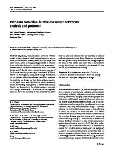
It is obvious that the number of hops does not affect the Efficiency Improvement Ratio. However, we should observe that EIR does change based on the size of sensing data in each data packet. In Fig. 4, we show EIR as a function of D, the size of sensing data in each data packet. From this figure, the improved transmission efficiency of the ADF protocol is obvious, especially when data information size is small. In other words, the smaller the size of sensing data in a data packet is, the larger the efficiency improvement ratio. This is because, when the size of sensing data is smaller, the effect of eliminating addresses in each packet is more pronounced. When the size of sensing data is as small as 16 bits, our protocol can improve the efficiency with respect to 32-bit static addresses by almost 80 percent and by nearly 40 percent with respect to 16-bit static addresses. In addition, we can also observe that the larger the size of an address space, the lower the efficiency the protocol has and ADF can thereby achieve higher efficiency improvement ratio by eliminating them.
IV. Performance Evaluation
80 EIR wrt. 16−bit static address EIR wrt. 32−bit static address
EIR (%)
60 40 20 0
0
200
400
600 800 1000 Sensing data (bits)
1200
1400
1600
Fig. 4: Efficiency improvement ratio
Tab. 2: Transmission Efficiency Data(bits) Analytical Simulation Anal.(16) Simu.(16) Anal.(32) Simu.(32)
16 0.00652 0.00647 0.00470 0.00466 0.00367 0.00364
64 0.02236 0.02221 0.01677 0.01665 0.01342 0.01331
256 0.05693 0.05668 0.04697 0.04672 0.03998 0.03974
512 0.07673 0.07647 0.06717 0.06686 0.05965 0.05936
1024 0.09277 0.09254 0.08535 0.08509 0.07907 0.07880
Tab. 1: System parameters Parameter Two-dimensional area Total packets sent Number of sensors that send data Sensor transmission range Sensor carrier sensing range Inter-handshake/Intra-handshake Space Bandwidth Channel packet error rate (PER) Location of the sink
Values 200 × 200 m2 500 per sensor 3 per run 40 m 88 m 50µs/10µs 200 kbps 0.05 (200 m, 200 m)
We have implemented the ADF protocol using the NS2 (ns2.27) simulator [10] and performed simulations to evaluate its performance. In this evaluation, we first validate our model of transmission efficiency proposed in Section III. We then evaluate the data delivery performance of the ADF protocol, and compare it with the modified ADF protocols which use static addresses and the traditional data delivery mechanisms. Important system parameters are shown in Tab. 1 as suggested by the existing hardware for WSNs [12].
A. Model Validation In this subsection, we set up a 9 × 9 grid network in an attempt to validate our model of predicted transmission efficiency given in Equations (4), (5), and (6). Eighty one nodes are uniformly placed in a grid network, which consists of eighty sensors and one sink which is located at the upper right corner (200m, 200m). Three sensors which send CBR traffic are located at the lower left corner (0m,0m), the lower right corner (0m,200m), and the upper left corner (200m,0m). The size of data packet varies from 2 bytes to 128 bytes while CBR rate is fixed at 1 packet/second. As in the analysis, probability of channel errors is set to 0. Also, we set a field in the data packet header so that we can trace the number of hops a data packet travels and estimate the number of average hops from all the data packets received at the sink (Total number of hops/number of data packets received). Simulation results come from sensing data received at the sink divided by the total bits transmitted in the whole network while analytical results are calculated via Equations (4), (5), and (6). The results of this experiment are shown in Tab. 2 and the average number of hops is estimated to be around 9 hops. Note that we do not count physical layer overhead in the total number of bits transmitted both in analytical and simulation results. From the table, we note that simulation results are slightly lower than our analytical results. This is because of the packet collisions due to hidden terminals. Overall, a good
match has been observed between our simulation results and analytical results. Therefore, the simple model used in our analysis yields fairly accurate results under light traffic load that we simulated.
B. Data Delivery Performance In this subsection, we evaluate the data delivery performance of ADF in terms of Packet Delivery Ratio (number of nonduplicate data packets received at the sink/number of data packets generated by the sensors), Average End-to-End Packet Delay (average network latency of received data packets), and Normalized Overall Communication Overhead (total number of packets sent at the MAC layer/Packet Delivery Ratio). The baselines used for this comparison are a modified ADF using 16-bit static addresses (called ADF16), a modified ADF using 32-bit static addresses (called ADF32), and DSR over IEEE 802.11 [11] both with and without RTS/CTS exchange.8 Network topology and configuration in this experiment is almost the same as the 9 × 9 grid network in last subsection except that we set channel packet error rate (PER) to 0.05. In each run of simulation, there are 3 sensors sending 500 packets of size 32 bytes at a fixed rate to the sink, while the rate changes in different configurations from an initial 1 packet/second to 19 packets/second in steps of 2 packets/second. The simulation results are presented in Fig. 5. From these simulation results, we observe that ADF has a packet delivery ratio that is comparable to that of ADF16 and ADF32 while DSR/802.11 (whether RTS/CTS is on or off) loses packets early as it quickly congests the network by sending route discovery packets. When sensor transmission rates become sufficiently large to congest the network, the performance of DSR quickly degrades and it drops a large number of data packets due to the increased collisions between nodes and unstable routing information, especially when the RTS/CTS exchange is turned on. We also see that ADF has a lower average end-toend packet delay than ADF16 and ADF32 because ADF has fewer bits to transmit, which leads to lower transmission delay and retransmission delay due to a lower probability of packet collisions at every hop. Note that DSR has a much higher packet delay because of the delay induced by its route discovery phase. The simulation results demonstrate large communication overhead savings in ADF compared with DSR/802.11, 8 Although DSR over 802.11 is originally designed for ad hoc networks and it is not a good data delivery mechanism for WSNs, we use it as a baseline since this mechanism is state-based and node-identifer-based, perfectly opposite to the state-free and nodeidentifier-free features of ADF. Thus, we can observe and understand the effects and advantages of these two features of ADF as a whole from the simulation results.
4
1.8
0.9
1.6 0.8
3.5 ADF ADF16 ADF32 DSR over 802.11 without RTS/CTS DSR over 802.11 with RTS/CTS
1.4 Average Delay (ms)
Packet Delivery Ratio
5
x 10
Normalized Overhead (number of packets)
2
1
0.7 0.6 0.5
1.2 1 0.8 0.6
0.4 0.3 0.2 0
ADF ADF16 ADF32 DSR over 802.11 without RTS/CTS DSR over 802.11 with RTS/CTS 5 10 15 Sensor CBR Traffic (packets/second)
0.4
x 10
3
ADF ADF16 ADF32 DSR over 802.11 without RTS/CTS DSR over 802.11 with RTS/CTS
2.5
2
1.5
1
0.2
20
0 0
(a) Packet Delivery Ratio
5 10 15 Sensor CBR Traffic (packets/second)
(b) Average End-to-End Delay
20
0.5 0
5 10 15 Sensor CBR Traffic (packets/second)
20
(c) Normalized Overhead
Fig. 5: Simulation results for a 9 × 9 grid network
which has to use a large number of routing and Address Resolution Protocol (ARP) packets. As expected, ADF has a lower communication overhead than ADF16 and ADF32 due to fewer packet collisions and data re-transmissions. To sum up, our simulation results show that ADF has no performance loss and even performs better than ADF16 and ADF32 since fewer bits transmitted in ADF can lead to lower probability of packet collisions and lower packet transmission delay. Our results also demonstrate performance advantages of our protocol over traditional data delivery mechanisms without state-free and node-identifier-free features, DSR over 802.11 in this evaluation, for example.
V. Conclusions We have presented a data delivery protocol ADF, which combines the tasks of forwarding and MAC via cross-layer design, for address-free WSNs. In ADF, receivers at every hop compete for the data forwarding task so that sensors are not required to maintain states of other sensors. Our protocol exploits the distance information and the broadcast nature of the wireless medium to complete the broadcast handshake at every hop and thereby removes the need for sensor identifers from packets. Using a simple analytical model, we quantified the transmission efficiency of ADF. Our analysis, validated by simulations, shows that ADF enjoys a rather high transmission efficiency gain by eliminating sensor identifiers. Our simulations performed in NS2 also show a higher packet delivery ratio and lower end-to-end delay and overall communication overhead in an example grid network, compared with ADF16 (the same forwarding strategy as ADF while employing 16bit static addresses), ADF32 (the same forwarding strategy as ADF while employing 32-bit static addresses), and DSR over 802.11. These simulation results demonstrate that ADF has a performance advantage over them due to its intrinsic state-free and node-identifier-free features. Our future research work will include a refined analysis of transmission efficiency which can predict the average number of hops in a randomly deployed sensor network and can take channel errors and hidden terminal problem into account. In addition, we will perform a comprehensive protocol performance analysis, comparison, and study of ADF with other existing data delivery mechanisms through analytical and simulation methods.
Acknowledgments This work was supported in part by the SUPRIA program of the CASE center at Syracuse University.
References [1] G. Pottie and W. Kaiser, “Wireless Integrated Network Sensors,” in Communications of ACM, Vol. 43, No. 5, pp. 51-58, May 2000. [2] J. Elson and D. Estrin, “Random Ephemeral Transaction Identifiers in Dynamic Sensor Networks,” in Proceedings of ICDCS21, Arizona, April 16-19, 2001. [3] M. Zorzi, R.R. Rao, “Geographic Random Forwarding (GeRaF) for Ad Hoc and Sensor Networks: Multihop Performance,” in IEEE Trans. on Mobile Computing, vol. 2, Oct.-Dec. 2003. [4] B. M. Blum, T. He, S. Son, and J. A. Stankovic, “IGF: A Robust State-Free Communication Protocol for Sensor Networks,” in Technical report CS-2003-11, CS Department, University of Virginia, 2003. [5] D. Chen, J. Deng, and P. K. Varshney, “A State-Free Data Delivery Protocol for Wireless Sensor Networks,” in proceedings of IEEE WCNC 2005, New Orleans, LA, USA, March, 2005. [6] C. Intanagonwiwat, R. Govindan, and D. Estrin, “Directed Diffusion: A Scalable and Robust Communication Paradigm for Sensor Networks,” in Proc. of MobiCom 2000, Massachusetts, August 2000. [7] Fan Ye, Gary Zhong, Songwu Lu, Lixia Zhang, “GRAdient Broadcast: A Robust Data Delivery Protocol for Large Scale Sensor Networks,” accepted by ACM WINET (Wireless Networks). [8] Andreas Savvides, Chih-Chieh Han, and Mani B. Strivastava, “Dynamic Fine-grained Localization in Ad-Hoc Networks of Sensors,” Proc. of MobiCom 2001 , Rome, Italy, July 16-21. [9] N. Bulusu, J. Heidemann, and D. Estrin, “GPS-less Low Cost Outdoor Localization For Very Small Devices,” IEEE Personal Communications Magazine, 7(5), pp. 28-34, Oct. 2000. [10] K. Fall and K. Varadhan, “The NS Manual,” UC Berkeley, LBL, USC/ISI, Xerox PARC, 2002: http://www.isi.edu/nsnam /ns/. [11] “IEEE Standard for Wireless LAN - Medium Access Control and Physical Layer Specification, P802.11,” 1999. [12] “XBOW MICA Mote Specifications,” http://www.xbow.com/ Products/products.htm.