Abstract A number of wireless sensor network (WSN) applications demand ... trol mechanisms to ensure timely data delivery and reliability control mechanisms.
Time-Critical Data Delivery in Wireless Sensor Networks Petcharat Suriyachai, James Brown, Utz Roedig Lancaster University, UK, {p.suriyachai, j.brown, u.roedig}@lancaster.ac.uk
Abstract A number of wireless sensor network (WSN) applications demand timely data delivery. However, existing WSNs are designed to conserve energy and not to support timely data transmission. This paper shows how WSNs can be dimensioned, deployed and operated such that both reliable and timely data delivery is ensured while scarce energy is preserved. The presented solution employs a novel Medium Access Control (MAC) protocol that incorporates topology control mechanisms to ensure timely data delivery and reliability control mechanisms to deal with inherently fluctuating wireless links. An industrial process automation and control scenario at an oil refinery in Portugal is used to define protocol requirements. The paper details a TinyOS implementation of the protocol and its evaluation in a testbed. Under high traffic load, the protocol delivers 100% of data in time using a maximum node duty cycle as little as 2.48%. In an idle network a maximum node duty cycle of only 0.62% is achieved. This proposed protocol is thus an extremely energy efficient solution for time-critical data delivery.
1 Introduction Future application areas of wireless sensor networks (WSNs) may include industrial process automation, aircraft control systems or traffic management systems. In such systems, the WSN is part of a control loop, and predictable network performance in terms of message transfer delay and reliability is required. To construct functioning control loops, it is necessary to ensure that sensor data is transported within a given time bound D. If too much sensor data arrives late or not at all due to losses on the wireless links, the control loop is unable to function. Data needs to be transported to the decision point (normally the sink) within a given time DS . Thereafter, a command needs to be transferred within a given time DA from the sink to an actuator. DA might be zero if the actuator is located at the sink. Data arriving late cannot be used in the decision process and has to be considered lost. Early data delivery is acceptable but not desirable as it implies that resources are used inefficiently. Instead of delivering data early, the network may spend these resources to improve transmission reliability or energy consumption of nodes. This paper presents a MAC protocol that is capable of supporting applications with the previously outlined communication requirements. The novel TDMA-based Medium Access Control (MAC) protocol incorporates routing, topology control and reliability control mechanisms to achieve the set goals. This protocol assumes that a small and relatively static network with predictable traffic patterns is deployed in a known environment. These assumptions hold true for the target area of industrial process automation and control. A network wide transmission schedule is determined before network
deployment, ensuring collision free and timely data delivery. During network operation reliability control mechanisms are employed to cope with fluctuating characteristics of the wireless channel. Designing a protocol with the outlined performance goals in wireless communication is very challenging. The protocol must be able to provide stable data transport performance using non-deterministic wireless links. Such performance is the main design goal, but energy consumption cannot be neglected as a reasonable network lifetime must be achieved. Moreover, the protocol should not be too complex so that it can be debugged easily and executed on resource constraint nodes. Finally, the protocol should allow flexibility to enable the addition of new nodes and minor topology changes. The paper gives a description of a real deployment scenario for which the protocol is designed: industrial process automation and control for an oil refinery in Sines, Portugal. This scenario and its requirements motivate the development of the communication protocol described and evaluated in this paper. The main contributions of the paper are: – GinMAC: A novel TDMA-based MAC protocol called GinMAC is presented, and details of its implementation on TinyOS for TelosB nodes are provided. – GinMAC Evaluation: The testbed evaluation validates that GinMAC can support the target industrial process control and automation applications. The delay and reliability requirements are met while achieving extremely low duty cycles, leading to an acceptable network lifetime. – Delay Conform Reliability Control: GinMAC incorporates a variety of strategies to deal with inherently non-deterministic wireless links while adhering to the given delay requirements. The effectiveness and associated energy cost of the different reliability control strategies are evaluated and discussed. The paper is organized as follows. Section 2 describes an industrial process control and automation scenario which demands a protocol such as GinMAC. The analysis of this real application scenario defines our network assumptions and requirements. Section 3 provides a detailed description of GinMAC. Section 4 presents an evaluation of GinMAC. Section 5 reports on related work dealing with the deployment of timecritical sensor networks. Section 6 concludes the paper.
2 Assumptions, Requirements and Problem Definition Most industrial process control and automation applications can be considered timecritical. In these scenarios, control loops are mapped onto wireless sensor networks. For such control loops to function, data needs to be delivered reliably and within a given time bound [1]. Furthermore, it might be necessary to react upon the received data, and a command needs to be delivered reliably and within a given time bound from the sink to an actuator in the sensor network. As WSNs are considered to be relatively unreliable, they so far have seen little use for such tasks. However, given the large cost savings due to a wireless deployment in industrial settings, the feasibility of wireless process control and automation is recently investigated. In this section, we use the GALP oil refinery at Sines, Portugal as an example scenario for industrial process control and automation. Oil refineries employ a large number of sensors to monitor their processes. Cabling cost is the main expense in installing
Figure 1. The GALP oil refinery in Sines, Portugal and deployed sensors/actuators.
such systems. Moreover, cabled control systems are inflexible as installation time is needed whenever production processes must be added or modified. Thus, it is desirable to utilize WSNs as base for such control systems to circumvent this hurdle. We visited the GALP oil refinery and spoke to technicians who have installed and maintained the currently cabled process automation and control systems to identify system requirements of a WSN. 2.1 The GALP Refinery Application Scenario The GALP oil refinery at Sines, Portugal is a complex industrial facility that includes a wide range of processing, and such processing needs careful monitoring and control of operations. There are currently 35000 sensors (some shown in Figure 1) and actuators in use in the refinery to perform real-time monitoring of industrial operations such as leakage detection and measurement of pressure in the pipes, fluid levels and of the overall environment. The monitoring of the environment in a refinery provides essential information to ensure the good health of both the refinery and its production processes. In such a typical section of the distribution system, a number of system conditions need to be closely monitored by sensors: – Pressure is monitored within each pipe not only for safety reasons to keep pipe pressure within pipe tolerances but also to detect leakage and derive flow information. Pressure is usually measured in Pascals. A typical pressure sensor can use a 32bit sample size. Pressure is typical sampled at a frequency of f = 1Hz. – Temperature is monitored within each pipe and tank for safety reasons. In addition, it is measured in degrees Celsius (C) at a typical frequency of f = 1Hz with a sample size of 32bits. – Shut-off valves are monitored to ensure that they are in functioning condition when needed, and they are periodically partially closed to check that the closing mechanism is operational. Valve status can be encoded as 8bit value. The value is sent periodically ( f = 3 · 10−3Hz), which can be adjusted by plant technicians. The plant also has a number of actuator systems that can be directly controlled from the refineries control center. These actuators include the following: – Shut-off valves are integrated into pipes and are used to interrupt product flow during day to day operations and in the case of emergency.
– Pumps can operate at different speeds to increase or decrease the pressure and thus flow of product through the piping system. Sensor samples should be transported to the control center within a few seconds. The exact delay requirement depends on the production process, but delay bounds of up to DS = 1s are required. Likewise, actuators must be reached within a few seconds, and a delay bound of DA = 1s is a typical value. All data losses should be avoided, but small loss rates in the order of 0.01% are deemed to be acceptable within control loops. 2.2 Assumptions and Requirements The example refinery deployment can be used to determine which assumptions can be made and which requirements a WSN has to fulfill. The requirements and assumptions are derived from the investigated refinery process control and automation application. However, we are confident that other large scale production facilities have very similar structures, and therefore the communication protocol presented in this paper is valid for not only the outlined application scenario but also other similar scenarios. Deployment: Sensors and actuators are installed at carefully chosen positions. It is possible to change their location slightly by a few meters during deployment. During operation nodes are static and do not move. In addition, the physical environment is fairly static as well. Thus, sensor nodes equipped with wireless radios can be positioned such that reasonable connectivity to a neighboring node is given. It is also possible to determine worst-case and best-case link reliability during deployment phase of the network. Maintenance: Most sensors can be mains powered, but some sensors may still be battery powered. Thus, energy consumption patterns are important but not necessary for all nodes. Sometimes additional sensors are deployed only for a few days to collect additional data. The network must consequently provide some degree of flexibility. Topology: The refinery has a large number of in-field control stations which are interconnected by a cabled network and have a power supply. All in-field control stations forward data to the main refinery control room. The in-field control stations are currently used to aggregate data from cabled sensors and actuators in their vicinity. If a WSN is used, the in-field control station can act as a sink to which sensors and actuators in the vicinity connect via wireless communication. An in-field control station manages up to N = 25 nodes. Most nodes will be located one hop from the sink (determined by on-site experiment) and at most a distance of 3 hops will be observed. All nodes controlled by one in-field control station can use one frequency, while neighboring in-field control stations use another transmission frequency. It is feasible to put nodes in the refinery in small clusters that are interconnected via the in-field control stations by a cabled network. Traffic: Nodes might report data frequently with a relatively high data rate (up to f = 1Hz). However, the packet payload can be considered to be quite small. Data is expected to reach the sink within a given time bound DS . This time bound can be expected to be in the order of a few seconds; the tightest bound of DS = 1s must be considered. The commands sent from the sink to actuators must arrive within a given time bound DA which can be as low as DA = 1s. The sink might also send commands to sensor node to
set sampling frequencies and to issue other configuration commands. These command messages may not need to be delivered within a given delay bound. The traffic patterns of the nodes in the network are reasonably known at deployment time.
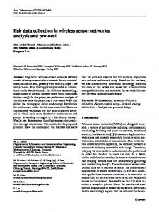
3 Time-Critical Data Delivery With GinMAC With the the target application domain and its requirements in mind, we choose to implement the following main features in GinMAC: 1. Off-line Dimensioning: Traffic patterns and channel characteristics are known before network deployment. Thus, complex protocol operations such as calculation of the transmission schedule is performed off-line and before network deployment. 2. Exclusive TDMA: Only a small number of nodes (N ≤ 25) need to be accommodated. Nodes are placed close to each other, and a high level of interference can be expected. A TDMA schedule with exclusive slot usage is consequently selected. 3. Delay Conform Reliability Control: The protocol must support delay bounds of DS and DA while achieving very high data transport reliability. Hence, all available flexibility in transport delays is used to improve reliability, given that our energy consumption target permits. 3.1 Off-line Dimensioning A network dimensioning process is carried out before the network is deployed. The input for the dimensioning process are network and application characteristics that are known before deployment. The output of the dimensioning process is a TDMA schedule with frame length F that each node has to follow. The GinMAC TDMA frame consists of three types of slots: basic slots, additional slots and unused slots. First, the frame contains a number of basic slots which are selected such that within frame length F each sensor can forward one message to the sink and the sink can transmit one message to each actuator. Second, the GinMAC frame uses additional slots to improve transmission reliability. Finally, the frame may contain unused slots which are purely used to improve the duty cycle of nodes. The above types of slots within the GinMAC frame must be designed such that the delay ( F < min{DS , DA }), reliability and energy consumption requirements are met. However, it may not always be possible to find a frame that simultaneously fulfills all three requirements. If that is the case, some dimensioning assumptions must be relaxed. To determine the number of basic slots required in a GinMAC frame, a topology envelope is assumed. This topology envelope is specified as a tree rooted at the sink and described by the parameters: maximum hop distance H and fan-out degrees Oh (0 ≤ h ≤ H) at each tree level h; we define O0 = 1. The topology envelope can accommodate a n maximum number of N max = ∑H n=1 ∏m=1 Om nodes. However, in the actual deployment max a number of nodes N ≤ N may be used. Nodes in the later deployment can take any place in the network and even move as long as the resulting deployed topology stays within this topology envelope. The maximum number of sensor nodes NSmax and actuator nodes NAmax (with N max = NSmax + NAmax ) must also be known.
Level 0 N-0-0-0 (SINK) N-1-0-0
Level 1 (O=4)
N-2-0-0
Sink Possible node position
N-1-1-0
N-1-2-0
N-1-3-0
N-2-1-0
N-2-2-0
N-2-3-0
Level 2 (O=3)
Sensor in deployment Actuator in deployment
Level 3 (O=2) N-1-1-1
N-1-1-2
N-1-2-1
N-1-2-2
N-1-3-1
N-1-3-2
N-2-1-1
N-2-1-2
N-2-2-1
N-2-2-2
N-2-3-1
N-2-3-2
Figure 2. Example topology with NA = 2 actuators and NS = 10 sensors.
To determine the number of additional slots needed for reliability control, the worstcase link characteristics in the deployment area must be known. As the network is deployed in a known environment, it is possible to determine this value by measurement. The configuration of basic and additional slots determines an energy consumption baseline of nodes. Adding unused slots within the GinMAC frame can improve upon this baseline. Next, we present how to obtain the GinMAC frame configuration. 3.2 TDMA Schedule and Reliability Control GinMAC uses TDMA slots whose size is fixed and large enough to accommodate a data transmission of a maximum length and an acknowledgement from a receiver. Moreover, these slots are used exclusively; a slot used by one node cannot be re-used by other nodes in the network. The protocol therefore does not scale to networks with many nodes. However, as described in Section 2, this scalability restriction is not an issue in the target application scenario. Furthermore, nodes are close together, resulting in high levels of interference that would limit potential slot re-usage. Finally, exclusive slot usage allows us to construct a protocol which is relatively simple to implement. Basic Slots: The topology envelope, which is defined by the maximum hop distance H and fan-out degrees Oh , is used to calculate the basic slot schedule within the GinMAC frame. An example topology envelope for H = 3 and O1 = 4, O2 = 3, O3 = 2 is shown in Figure 2; recall that we define O0 = 1. Basic slots SB are dimensioned under the assumption that all positions in the topology envelope will be occupied by nodes. The basic slots SB accommodate two different traffic flows. First, a number of basic slots SBup are required to accommodate traffic flowing from all nodes to the sink; we assume actuators might be used for sensing as well. Second, a number of basic slots SBdown are required to accommodate traffic flowing from the sink to actuators (SB = SBup + SBdown). A leaf node (level H) in the tree requires one basic TDMA slot within F to forward data to its parent node. This parent node requires a slot for each child node plus one slot for its own data for forwarding to its parent. Its slots must be located after the slots used by its children to ensure that data can travel within one GinMAC frame through the tree to the sink. The allocation of the transmission slots for the previously given topology is depicted in Figure 3. The total number of slots in F needed to forward up data to the sink SBup can be calculated as follows. A node at tree level h requires SB,h = up up up Oh+1 · SB,h+1 + 1 with SB,H = 1. Consequently, SB can be calculated as: SBup =
H
h
h=1
i=1
up · ∏ Oi ∑ SB,h
(1)
UPSTREAM SLOTS
N-4-3-0
N-4-3-0
N-4-2-0
N-4-2-0
N-4-1-0
N-4-1-0
N-4-0-0
N-4-0-0
N-3-3-0
N-3-3-0
N-3-2-0
N-3-2-0
N-3-1-0
N-3-1-0
N-1-2-0
N-3-0-0
N-3-0-0
N-1-0-0
N-1-2-2
N-1-3-0
N-2-1-1
N-1-3-2
N-1-2-0
N-1-3-1
N-1-2-2
N-1-1-0
N-1-2-1
N-1-1-2
N-1-1-1
S1 S2 S3 S4 S5 S6 S7 S8 S9 .........
DOWNSTREAM SLOTS
Figure 3. Transmission slot allocation for the topology shown in Figure 2.
In the topology shown in Figure 2, SBup = 100 is required. The sink must be able to send a data packet to each actuator within one GinMAC frame. Thus, the sink requires some slots for these actuators. The slot allocation for nodes at level h is the minimum between the maximum number of actuators (NAmax ) in the network and the number of nodes below this level h. The redown for each node at level h can be calculated as quired number of downstream slots SB,h H i down = 0. Hence, Sdown can be calculated as: down max SB,h = min{NA , ∑i=h+1 ∏ j=0 O j } with SB,H B SBdown =
H−1
h
h=0
i=0
down · ∏ Oi ∑ SB,h
(2)
In the topology shown in Figure 2 where there is a maximum of NAmax = 2 actuators in the network, SBdown = 34 is therefore required. There could be configuration commands from the sink to nodes. In this case, we assume that such commands are not time-critical. They thus can be broadcasted when there is no actuation command to send, reusing the slots provisioned for the actuators. Additional Slots: The basic slots can only assure data transport if no messages in the network are lost due to an erroneous wireless channel. However, in an industrial setting this erroneous channel is unavoidable, and consequently our protocol must provide some transmission redundancy. GinMAC employs the so-called additional slots SA to implement temporal and spatial transmission diversity. To determine the number of additional slots, we first need to choose a worst-case link reliability that GinMAC will support; the definition of reliability is elaborated in the next paragraph. The deployed system will form a topology that fits into the topology envelope and uses only links with reliability better than the selected worst-case link reliability. These links are called good links. Pre-deployment measurements are used to determine a reasonable value for the worst-case link reliability such that enough good links are available for topology formation. GinMAC monitors link reliability during operation and removes the links whose reliability becomes lower than the worst-case reliability threshold. We propose two methods for specifying good links. The first method simply uses the Packet Reception Rate (PRR). A good link is defined as having a PRR above a specific threshold. The second method applies burst lengths to define worst-case link reliability. A good link must not have more than Bmax consecutive transmission errors and must provide at least Bmin consecutive successful transmissions between two bursts. A recent study has shown that this definition captures link quality better than PRR [3].
Temporal Transmission Diversity: In a scenario where good links can be characterized with short Bmax and long Bmin , it is possible to efficiently add additional retransmission slots on the same link to deal with losses. Consider node N-1-1-0 in the example shown in Figure 2, Bmax = 2 and Bmin = 2. The node requires 3 basic slots for upstream transmissions, and in a worst case any 2 of the 3 transmissions might be lost. However, if 4 additional transmission slots are allocated, all 3 packets are guaranteed to be delivered within the 7 slots provided that the channel conforms to chosen Bmax and Bmin . The number of necessary additional slots SA,h per node at level h can be calculated as: SA,h =
�
� SB,h · Bmax Bmin
(3)
The additional upstream and downstream slots are added in the schedule directly after the respective basic slots for each direction. If a node fails to transmit data in a basic slot, it can use an additional slot for a retransmission. If links are good links as defined by Bmax and Bmin , all messages are delivered successfully and in time. There might be scenarios where only links can be found that have a relatively high PRR but simultaneously have a long Bmax and short Bmin . In this case, these links are generally of good quality, but sometimes transmissions are impossible for extended periods of time. Thus, SA,h would become excessively large, and the delay target may be violated as the GinMAC frame F might become too long. However, such scenarios could still be supported using temporal and spatial transmission diversity. Temporal And Spatial Transmission Diversity: It is possible to duplicate the basic schedule m times within a GinMAC frame if the overall delay goal permits. Nodes in the deployment are then able to join m + 1 topologies in which each of them adheres to the set topology envelope. When a node transmits a message, it sends a copy of the message in each of the m + 1 topologies. The concurrent topologies should be selected such that they do not use the same links whenever possible. The assumption is that copies of the same message use disjoint paths and are therefore not corrupted by infrequent but long burst errors on one link. The number of necessary additional slots SA,h per node at level h can be calculated as: SA,h = m · SB,h
(4)
The number m must be selected such that an acceptable high packet delivery rate to the sink and to actuators can be achieved. This temporal and spacial transmission diversity clearly costs much more energy than the temporal transmission diversity. Unused Slots and Energy Consumption: A GinMAC frame consisting of only basic and additional slots may be shorter than the delay requirements would allow ( F < min{DS , DA }). In this case, it is useful to add the so-called unused slots SU after the basic and additional slots such that F = min{DS , DA }. A node turns the transceiver off in these unused slots, and thus the energy consumption of a node is improved. The energy consumption of a node operating GinMAC can be calculated before network deployment. This calculation is useful in industrial deployments where maintenance schedules must be predictable. For each node position in the topology envelope, the worst-case and best-case energy consumption can be determined. The worst-case is
incurred if nodes use all assigned slots. In contrast, the best-case is incurred when nodes do not have to forward sensor data and only maintenance messages are transmitted. As GinMAC is a TDMA protocol, time synchronization is necessary. For this purpose, a node listens every k frames in the first slot that its parent node transmits data upstream. Thus, all nodes synchronize their time with the sink. Every node must always transmit (a packet without payload if no data is available) in the first slot used for upstream data. The packet header contains information on how many packets the sender has to transmit in the current GinMAC frame. Upon receiving the first packet, the receiver knows how many consecutive slots need to be activated for packet reception. If a node does not receive a packet in this first slot, a packet loss is assumed. The node then will listen in the next receive slot. A node might need to use provisioned additional slots to receive all messages. Moreover, a node must transmit in the first slot used to send actuator data to each child node if actuators are located downstream. Again, if a child does not receive data, it will assume a loss and listen in following slots for a retransmission. However, even if no actuators are located downstream, a node still needs to listen in the first downstream slot in case a parent node has to forward non time-critical control messages. If these control messages are lost, they will not be retransmitted within the same GinMAC frame. Best-Case Energy Consumption: We assume that a transceiver requires the same power p for transmission, reception and idle listening. The power also depends on the task carried out that determines how long a transceiver is active within a slot. The time t the transceiver is active determines the energy consumption e = p · t in a slot. It is assumed that within time tl the transceiver can determine that no transmission occurs; an acknowledged transmission of a packet without payload requires te ; the acknowledged transmission of a full packet requires t f with tl < te < t f 1 . The best-case energy consumption Ehbest of a node at level h in the topology that does not have to forward actuator data and uses either only basic slots or Temporal Transmission Diversity is obtained as: 1 Ehbest = (tl + ( + 1 + Oh+1) · te ) · p ∀h > 0 (5) k In the case that both Temporal and Spacial Transmission Diversity is used, the energy consumption baseline given by Ehbest must be multiplied by a factor of m + 1. Worst-Case Energy Consumption: If data is transmitted in all available slots, the worstcase energy consumption Ehworst of a node at level h in the topology is incurred as: 1 Ehworst = ( + 2 · (SB,h + SA,h) − 1) · t f · p k
∀h > 0
(6)
The duty cycle δh of a node at level h is defined as the relation of transceiver on time to total time and can be calculated as δh = Eh /(F · p). For example, assume retransmission slots are not needed, and thus SA,h = 0. The energy consumption of a node at level 1 in Figure 2 is E1best = (tl + ( 1k + 4) · te ) · p and E1worst = ( 1k + 23) · t f · p. If a CC2420 transceiver, a slot size of 10ms, a frame length of F = 1s and k = 100 are assumed, the duty cycles δ1best = 0.45% and δ1worst = 11.04% can be achieved. 1
For example, a CC2420 transceiver requires approximately the same power for transmission, reception and listening. It also uses task times of tl = 0.128ms, te = 1.088ms and t f = 4.800ms.
3.3 Topology Control A node added to the network must determine in which slots it must become active before it can transmit or receive data. The steps used to achieve this are described below. After a node is switched on, it must first obtain time synchronization with the network. Both control and data messages transmitted in the network can be used to obtain this time synchronization. The node continuously listens to overhear a packet from the sink or a node that is already operating in the network. After overhearing one message, the node knows when the GinMAC frame starts as each message carries information about the slot in which it was transmitted. As a next step, the node must find its position in the topology which must stay within the defined topology envelope. For this purpose, the new node listens for packets in all slots. Transmitted data packets use a header field in which a node that is already a member of the network advertises potentially available positions. For example, a node at position N-1-1-0 shown in Figure 2 may advertise in a header of a data packet traveling to its parent N-1-0-0 that position N-1-1-1 is available. The new node can claim an advertised position by transmitting a data packet in the slot allocated by the advertising node for a potential child node. If an acknowledgement for this transmission is received, the new node has successfully claimed this position in the topology. A node may be configured with a list of valid nodes that it is allowed to attach to. This might be necessary to ensure that a node will only attempt to join the network using known good links as determined by measurements before the deployment. If a node observes during operation that a link does not fulfill the criteria of a good link, it may decide to attach to the network using a different link. In such a case, a node changing position in the topology must inform its potential child nodes of this event. If a node looses connectivity to its parent node (determined by an unsuccessful data transmission within one GinMAC frame), it will fall back into the previously described pattern where a node listens on all slots to find a valid attachment point.
4 GinMAC Evaluation An evaluation is carried out to verify if GinMAC can fulfill the application requirements detailed in Section 2. The protocol is implemented on TinyOS 2.0.2 for TelosB nodes. 4.1 Setup Ideally, the evaluation should be carried out in an industrial environment such as the GALP oil refinery. However, due to health and safety regulations and possible interference with production, we were not yet able to carry out long-term in situ experiments. Thus, the evaluation testbed is deployed in a corridor of our office building. Nodes are placed on top of metal door frames in a corridor, and consequently communication links can have relatively high loss rates (up to 20%). Such link characteristics are present in the envisioned target scenario where metal pipework obstructs communication paths. The target platform uses a CC2420 transceiver, and a slot length of 10ms is selected. This slot size provides enough time to process and transmit a packet of a maximum payload size and to acknowledge this transmission using hardware acknowledgements. All
packets in the experiment have a size of 44bytes, and thus transmission, reception and listening task times are tl = 0.128ms, te = t f = 1.952ms, respectively. Time synchronization is obtained every k = 10 frames. The aim is to support a delay bound of DS = 1s and traffic rates of up to f = 1Hz. Nodes are forced into a static binary tree topology with depth H = 3 containing N = 15 nodes that use links defined as “good links” and by Bmax = 1 and Bmin = 1. The worst-case link reliability is found via pre-deployment measurements. The automatic topology formation, which is described in the previous section, is not used in this evaluation. In the experiments, three different configurations are evaluated: (Config A) basic slots only, (Config B) basic and additional slots with temporal transmission diversity, and (Config C) basic and additional slots with both temporal and spacial transmission diversity. (Config A) For this configuration, the number of basic slots SB = 34 with SBup = 34 and SBdown = 0 is used as the network for evaluation does not contain actuators. The system is provisioned such that a delay bound of DS = 1s can be provided. However, no mechanisms are in place to handle packet losses. SU = 66 unused slots are added to obtain a GinMAC frame size of F = 100slots, which translates with a slot size of 10ms to the required delay bound DS . In an idle network where there is no data traffic, a leaf node will have a best-case duty cycle of 0.21%. In contrast, under full traffic load where all nodes send a data packet every GinMAC frame, a node directly under the sink will incur a worst-case duty cycle of 2.56%. (Config B) In this configuration SB = 34 basic slots and SA = 34 additional slots are used to deal with the worst-case channel characteristic given by Bmax = 1 and Bmin = 1. If a transmission fails, additional slots are used for retransmission. SU = 32 unused slots are added to bring the GinMAC frame size to F = 100slots to provide a delay bound of DS = 1s. In an idle network, a leaf node will have a best-case duty cycle of 0.21%. If under full traffic load, a node directly under the sink will incur a worst-case energy consumption of 5.09%. (Config C) In this configuration SB = 34 basic slots and SA = 34 additional slots are used again. The additional slots are used to implement a second disjoint topology. Nodes transmit data using both binary tree topologies to compensate for losses. SU = 32 unused slots are added to bring the GinMAC frame size to F = 100slots to provide a delay bound of DS = 1s. In an idle network, a leaf node will have a best-case duty cycle of 0.41%. If under full traffic load, a node directly under the sink will incur a worst-case duty cycle of 5.09%. In all experiments, nodes emit data packets at the traffic rate f where (0.1Hz ≤ f ≤ 1Hz). The achieved duty cycle δ of all nodes and the message delivery reliability r at the sink are recorded. An experiment lasts for 15minutes for each traffic rate. In addition, five experiments are repeated for each traffic rate to find an average of the energy consumption and delivery reliability measurements. 4.2 Results Configuration A: Before evaluating the first configuration in the corridor deployment, a separate experiment setup on a table is carried out. The aim of this initial table top evaluation is to determine how the protocol performs in a setting with negligible link
Average Node Duty Cycle Data Delivery Reliability [%]
Average Node Duty Cycle [%]
Message Delivery Reliability 1.01
Table Deployment Corridor Deployment Worst-Case Best-Case
1.4
1.2
1
0.8
0.6
0.4
0.2
0
Table Deployment Corridor Deployment 100%
1
0.99
0.98
0.97
0.96
0.95 0.1
1
Message Generation Frequency f [Hz]
0.1
1
Message Generation Frequency f [Hz]
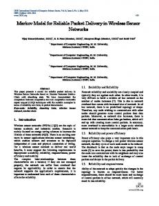
Figure 4. Average node duty cycle δ and reliability r using configuration A.
errors. In the table top deployment, all 15 nodes are placed in a grid with a spacing of 30cm , and the configuration similar to that in the corridor deployment is applied. Figure 4 presents the evaluation results for both table top and corridor deployments. These results are the average node duty cycle δ of all nodes, the average worst-case and average best-case duty cycles of all nodes, and the achieved delivery reliability r. The achieved duty cycles in both deployments are close to the theoretical best-case for low traffic loads and close to the theoretical worst-case for the maximum traffic rate of f = 1Hz. In the table top deployment, delivery reliability r is close to the desired reliability of 100% as transmission errors are rare. However, in the more realistic corridor deployment reliability can drop as low as 97.2% (one leaf node was found to have a high loss rate of 20%), resulting in an unacceptable performance for the applications described in Section 2. Nodes achieve slightly lower duty cycles in the corridor deployment as less data, due to transmission losses, is transported to the sink. Configuration B: Figure 5 shows the evaluation results for the deployment of configuration B. The delivery reliability is 100% which is desired for the target applications. Thus, the temporal transmission diversity in configuration B is able to compensate link errors seen in the configuration A. Although a price in terms of energy has to be paid to achieve improved reliability, in this case such cost was negligible as only a small number of retransmission slots were required over the duration of the experiment. Configuration C: Figure 5 depicts the evaluation results for the deployment of configuration C. The delivery reliability is 100% similar to that in configuration B, meeting the requirement of our target applications. However, this method is more costly in terms of energy than configuration B. The increase in energy consumption compared to configuration A is at most 0.53%.
4.3 Findings The evaluation shows that i) GinMAC can support the target application scenario and ii) the reliability control mechanisms as provided by GinMAC are essential to achieve the required high delivery reliability.
Average Node Duty Cycle Average Node Duty Cycle [%]
2.5
Corridor Deployment, Conf B Corridor Deployment, Conf C Worst-Case, Conf B and C Best-Case, Conf B Best-Case, Conf C
2
1.5
1
0.5
0 0.1
1
Message Generation Frequency f [Hz]
Figure 5. Average node duty cycle δ using configurations B and C.
Under the highest traffic load of f = 1Hz, the protocol can deliver 100% of data in time with a node duty cycle of at most 2.48%, as observed by nodes at level 1 in configuration B. The average node duty cycle δ of all nodes in this test scenario is only 0.76%. In an idle network a node duty cycle of at most 0.62% is achieved by nodes at level 1, while its average node duty cycle δ of all nodes is as little as 0.38%. Common MAC protocols aim for a duty cycle of approximately 2%, which increases with traffic load. Our evaluation illustrates that GinMAC matches this aim at a comparable duty cycle of 2.48% under high traffic load while providing timely and reliable data delivery. The presented implementation would allow for a number of optimizations. For example, sensor readings have only a size of a few bytes, but our 10ms slots can accommodate much larger packet sizes. Thus, a number of data readings could be transmitted within one slot, which would reduce the number of slots per level. Such an optimization would enable us to conserve more energy or to achieve much tighter delay bounds.
5 Related Work The WSN research community has to date produced a number of solutions addressing timely data delivery in wireless sensor networks [4]. However, most of these proposals do not completely match the requirements outlined in Section 2. Recent work highlights their shortcomings and points out that more research in this domain is required [2]. Closest to the presented work is the WirelessHART [5] protocol, which is specified by the HART communication foundation. WirelessHART is designed to support industrial process and automation applications. In addition, WirelessHART uses at its core a synchronous MAC protocol called TSMP [6], which combines TDMA and Frequency Division Multiple Access (FDMA). A central entity called Network Manager is used to assign collision free transmission slots and to select redundant routing paths through a mesh network. Thus, the protocol guarantees an upper delay bound while ensuring high transport reliability. Our protocol uses off-line dimensioning to circumvent the complexity and communication overheads that are introduced by this Network Manager. Prabh [7] specifies a TDMA-based MAC protocol for constructing a network that is dimensioned using scheduling theory. The protocol assumes that a network layout is in a hexagonal shape and that only neighboring nodes in the topology interfere. Based
on these assumptions, a carefully designed schedule is devised to achieve the minimum possible bound on message transfer delay. GinMAC is more flexible in terms of topology, and Prabh’ s methods are evaluated using only simulations. Dwarf [8] uses unicast-based partial flooding which limits the degree of transmission redundancy to preserve energy while maintaining reliability. In contrast to our work, all nodes are categorized into rings based on their distance to the nearest sink. The protocol selects a fixed number of forwarding neighbors according to their ring level and wake-up times to decrease an end-to-end delay. When retransmission is needed, a packet is resent to a different forwarding neighbor.
6 Conclusion The paper details GinMAC that achieves time-critical data delivery in WSNs with extremely low energy expenditure. Hence, the protocol can support industrial process automation and control applications required in the outlined GALP case study. Our evaluation shows that the reliability control mechanisms are practical and essential to deliver the high reliability requirement. In particular, these mechanisms of GinMAC allow us to balance delay, reliability and energy consumption requirements before network deployment. Such achievement is needed for carefully planned industrial control networks. Our next step is to evaluate GinMAC in a deployment at the GALP refinery. Acknowledgement This work has been partially supported by the European Commission under the FP7 contract FP7-ICT-224282 (GINSENG).
References 1. F.L. Lian, J. Moyne, D. Tilbury, “Network Design Consideration for Distributed Control Systems,” IEEE Trans. Control Syst. Technol., vol. 10, pp. 297-307, Mar. 2002. 2. A. Willig, “Recent and Emerging Topics in Wireless Industrial Communications: A Selection,” IEEE Trans. Ind. Informat., vol. 4, pp. 102-124, May 2008. 3. S. Munir, S. Lin, E. Hoque, S. Nirjon, J. Stankovic, K. Whitehouse, “Addressing Burstiness for Reliable Communication and Latency Bound Generation in Wireless Sensor Networks,” in Proc. 9th Int. Conf. Information Processing in Sensor Networks, Sweden, Apr. 2010. 4. J. Stankovic, T. Abdelzaher, C. Lu, L. Sha, J.Hou, “Real-time communication and coordination in embedded sensor networks,” Proc. IEEE, vol. 91, pp. 1002-1022, Jul. 2003 5. HART Communication Foundation, WirelessHART Data Sheet, [Online]. Available: http://www.hartcomm.org/, Apr. 2010. 6. K.S.J. Pister, L. Doherty, “TSMP: time synchronized mesh protocol,” in Proc. IASTED Symp. Parallel and Distributed Computing and Systems, Orlando, FL, USA, 2008. 7. K. Shashi Prabh, “Real-Time Wireless Sensor Networks,” Ph.D. Thesis, Department of Computer Science, University of Virginia, Charlottesville, VA, USA, 2007. 8. M. Strasser, A. Meier, K. Langendoen, P. Blum, “Dwarf: Delay-aWAre Robust Forwarding for Energy-Constrained Wireless Sensor Networks,” in Proc. 3rd IEEE Int. Conf. Distributed Computing in Sensor Systems, Santa Fe, NM, USA, 2007, pp. 64-81.