Hindawi Mathematical Problems in Engineering Volume 2017, Article ID 9852063, 10 pages https://doi.org/10.1155/2017/9852063
Research Article Efficient Data Mining Algorithms for Screening Potential Proteins of Drug Target Qi Wang, JinCai Huang, YangHe Feng, and JiaWei Fei Science and Technology on Information Systems Engineering Laboratory, College of Information System and Management, National University of Defense Technology, Changsha, Hunan, China Correspondence should be addressed to YangHe Feng;
[email protected] Received 9 December 2016; Revised 22 January 2017; Accepted 16 February 2017; Published 2 March 2017 Academic Editor: Stefan Balint Copyright © 2017 Qi Wang et al. This is an open access article distributed under the Creative Commons Attribution License, which permits unrestricted use, distribution, and reproduction in any medium, provided the original work is properly cited. The past few decades have witnessed the boom in pharmacology as well as the dilemma of drug development. Playing a crucial role in drug design, the screening of potential human proteins of drug targets from open access database with well-measured physical and chemical properties is a task of challenge but significance. In this paper, the screening of potential drug target proteins (DTPs) from a fine collected dataset containing 5376 unlabeled proteins and 517 known DTPs was researched. Our objective is to screen potential DTPs from the 5376 proteins. Here we proposed two strategies assisting the construction of dataset of reliable nondrug target proteins (NDTPs) and then bagging of decision trees method was employed in the final prediction. Such two-stage algorithms have shown their effectiveness and superior performance on the testing set. Both of the algorithms maintained higher recall ratios of DTPs, respectively, 93.5% and 97.4%. In one turn of experiments, strategy1-based bagging of decision trees algorithm screened about 558 possible DTPs while 1782 potential DTPs were predicted in the second algorithm. Besides, two strategy-based algorithms showed the consensus of the predictions in the results, with approximately 442 potential DTPs in common. These selected DTPs provide reliable choices for further verification based on biomedical experiments.
1. Background In domains of biotechnology, pharmacology, and medicine development, identification of drug targets is to discover new candidate molecules that are active in the process of remedies with drugs. A notation is given in [1] that the drug target is a broad concept ranging from molecular entities such as Ribonucleic Acids (RNAs), genes, and proteins to biological phenomena like phenotypes or pathways. History about the drug development has confirmed a fact that most failures in drug exploration can be attributed to inappropriate targets pursued [2, 3]. It is widely acknowledged that identifying potential targets for intervention is the first and foremost step in the modern drug campaign [1, 4–7], which has attracted increasing attention and focus from both academia and industry. Once the molecule was predicted as drug target, the engineering of drug design would begin in clinical trials. Since such programs, involving huge investments from pharmaceutical corporations and governments,
are exactly time-consuming and labor-intensive, the choice of potential targets for experiments seems quite crucial. As the dataset collected in our experiments is trapped in a special case where limited drug target proteins are known while the rest are uncertain in labels, the screening of potential drug target proteins from the unlabeled is complicated. A prior information supported in our research lies in low ratio of “druggable” genomes in humans, approximating to 10% [8]. In the light of this, the nondrug target proteins (NDTPs) would dominate the unlabeled by inference. For more detailed information about our dataset, see Materials and Methods, and our ultimate objective is to screen several reliable drug target proteins (DTPs) from the unlabeled. Looking back to the previous methodologies of identification of drug target proteins (IDTPs), some specific biological hypotheses were required such as side-effect similarity [9], chemical structure, and genomic sequence information [10]. For further review about this, refer to [4]. To overcome the limits on the reliability of hypothesis and explore a robust
2
Mathematical Problems in Engineering
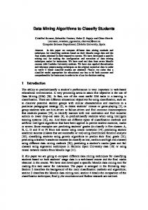
Microarray data
Data mining technique
Candidates list
Preclinical test
Expert decision
5376 unlabeled proteins 517 known DTPs
Figure 1: Process of drug target discovery using data mining techniques. Properties: 31 continuous, 5 nominal
way to address the problem as well, we have developed a novel paradigm combining the proteins biochemical characteristics with the booming data mining techniques. Figure 1 shows the process of drug discovery using data mining techniques. Inspired by a family of algorithms with regard to the positive and unlabeled learning, we transferred the existing knowledge into the domain of bioinformatics. A two-stage paradigm was adopted for the screening task, with the final result showing the efficiency of our algorithms.
2. Materials and Methods
Figure 2: Information about proteins with properties.
dataset with 517 known DTPs and 5376 uncertain NDTPs was employed for the screening task. Specifically, some proteins in the 5376 proteins would be recommended as most likely DTPs from the dataset of uncertain NDTPs. Further information about the dataset for experiments is illustrated in Figure 2 and supporting materials are in the website http://pan .baidu.com/s/1pLDCkcF.
2.1. Data Collection and Preliminary Analysis 2.1.1. Data Collection. Proteins, as one of the main sources of drug targets, have been a lasting heated topic for researchers from various domains. Some of them interact with each other, forming the basis of signal transduction pathways and transcriptional regulatory networks. As the focus of our research, proteins of drug targets are those functional biomolecules addressed and controlled by some active compounds. In this paper, we collected proteins from the DrugBank Database (Version 3.0) in which 1604 proteins were annotated as drug targets [11]. Further data cleaning was imposed by removing the nonhuman proteins as well as those sequences larger than 20% using PISCES [12]. As the compounds of atoms and molecules, whether the protein can be the candidate for the drug targets is frequently determined by factors like water solubility, hydrogen ion concentration (pH), trait of bases, and its structure. Though the interaction relations provide the additional information for the screening, they are not exactly reliable. Other properties of proteins also originate from the basic chemical or physical properties of proteins in essence. Our selected properties in the research were just some basic chemical or physical properties of proteins. We followed the extracting process in [13]. Then some properties of significance for our task were extracted such as peptide cleavages [14], N-glycosylation [15], O-glycosylation [16], low complexity regions [17], transmembrane helices [18], and some other influential physical or chemical characteristics. These properties were important clues in deciding the biological activity of proteins. We made use of pepstats, an online software from EMBOSS [19], to calculate statistics of properties. In our article, we also call the unlabeled proteins as uncertain NDTPs because of the former prior information about the proportions of DTPs in dataset. The uncertain NDTPs were those when we did not know whether any of them would be the drug target candidates. Finally, a collected
2.1.2. Preliminary Analysis. To eliminate the effect of scales, we impose normalization on each continuous property at first. The detailed process is as follows: 𝑧𝑖 =
𝑥𝑖 − 𝜇 , 𝜎
(1)
where 𝑧𝑖 is the normalized value of some property 𝑥𝑖 , 𝜇 is the mean of the population, and 𝜎 is the standard deviation of the property. After the preprocessing, we need to apply hypothesis tests to check whether the information of each property is beneficial for our screening task. More specifically, Kolmogorov-Smirnov two-sided test was picked as the technique while the DTPs and the unlabeled were recognized as two classes. Since the unlabeled were dominated by the NDTPs, it was reasonable to consider that the traits of the NDTPs can be well approximated by the distribution of the unlabeled with some noise from the potential DTPs. We denote the list of properties in the following order: Ala, Cys, Asp, Glu, Phe, Gly, His, Ile, Lys, Leu, Met, Asn, Pro, Gln, Arg, Ser, Thr, Val, Trp, Tyr, Tiny, Small, Aliphatic, Aromatic, Nonpolar, Polar, Charged, Basic, Acidic, Hydrophobicity, SignalP, LowComplexityRegions, Ogly S, Ogly T, Ngly, and Trans Helices. All of these have been elaborated in the former work [13] with the detailed process of property extraction. The final results in Table 1 show the difference of significance between two classes, suggesting almost all of these properties in our dataset are discriminating and the effectiveness of properties would further support the following experiments. Another factor would affect the predicting performance is the correlation between the properties. After computing the values of correlation, covariance matrix is visualized in Figure 3. In the figure, the names of the horizontal axis are just in the order of the list of properties from the top to the bottom as well as from left to the right in axes. As is
Mathematical Problems in Engineering
3 1.0 0.8 0.6 0.4 0.2 0.0 −0.2 −0.4 −0.6 −0.8
Figure 3: Correlation graph. If the color is darker enough, it means the rather stronger correlation between two properties.
shown in the figure, the properties have weak correlations between each other, indicating less information redundancy in the properties. Up to now, it seems that the task is able to learn since the properties are quite information-beneficial. Something must be emphasized that we only make use of continuous properties in our experiments to relieve the dimension disaster which comes from the nominal properties. Further experimental results would confirm our induction. 2.2. Two-Stage Methodologies. Taking details into consideration, an arduous task is the identification. The task is just a problem of one class classification, which is also viewed as the type of transductive learning [20]. If we want to establish a classifier, some negative samples, NDTPs, are in necessity. Here, we innovatively employ anomaly detection techniques [21] to convert the problem of one class classification to the general binary classification problem. Therefore, the task is addressed in the two-stage paradigm. Specifically speaking, the first stage is to screen some reliable negative ones for the formation of training dataset in the binary classification and then a classifier is constructed with the help of obtained dataset in the second stage. The flowchart in Figure 4 illustrates our framework in detail. 2.2.1. Strategies in the First Stage. The construction of the negative from the collected unlabeled is a nontrivial task and in some sense, it is to screen some reliable NDTPs. Though a prior knowledge indicates NDTPs’ large occupation in the unlabeled, the discriminating criteria between two classes are hard to make up. Here, some statistical analyses with proper techniques are employed for NDTPs’ fine extraction and we devise two strategies for the choice of reliable NDTPs from the perspective of statistical anomaly detection. Both of them are mining the inner discrimination between distributions of DTPs and the uncertain NDTPs. Strategy 1. Such strategy is in a nonparametric style and the computations in the initial process only rely on the
Table 1: Statistical results after K-S test. Most of properties are significant during test. Property Kolmogorov-Smirnov 𝑍 test Significance Ala 2.540 0.000 Cys 2.116 0.000 Asp 2.830 0.000 Glu 2.501 0.000 Phe 4.267 0.000 Gly 4.098 0.000 His 0.850 0.465 Ile 3.958 0.000 Lys 2.102 0.000 Leu 1.981 0.001 Met 2.765 0.000 Asn 3.154 0.000 Pro 3.625 0.000 Gln 4.481 0.000 Arg 2.845 0.000 Ser 5.161 0.000 Thr 1.481 0.025 Val 4.472 0.000 Trp 1.745 0.005 Tyr 5.011 0.000 Tiny 1.708 0.006 Small 1.598 0.012 Aliphatic 3.672 0.000 Aromatic 3.992 0.000 Nonpolar 4.908 0.000 Polar 4.908 0.000 Charged 2.252 0.000 Basic 3.065 0.000 Acidic 2.191 0.000 Hydrophobicity 1.908 0.001 SignalP 1.728 0.005 LowComplexityRegions 1.803 0.003 Ogly S 1.172 0.128 Ogly T 1.004 0.266 Ngly 2.667 0.000 Trans Helices 1.632 0.010
known DTPs. Here 31 continuous properties are just the decisive factors. Each property of proteins provides us with measurable criteria for selecting reliable NDTPs. An intuitive way is to characterize the extent of sample’s violating the statistical indexes or patterns displayed in the dataset of known DTPs. The range of the property where DTPs occupy in a higher probability can be restricted based on the quantile information on the accumulated distribution of the known DTPs and those proteins whose values of the property fall out of the range are more likely to share similar patterns with the reliable NDTPs. In our experiments, the reliable range for the DTPs regarding one continuous property is defined as an interval
4
Mathematical Problems in Engineering The flowchart of our framework
Uncertain NDTPs waiting for testing
DTPs
Rough identification First stage algorithms
Final identification
Reliable NDTPs The rest of uncertain NDTPs
DTPs
Second stage algorithm Model training Classifier establishment
Figure 4: Flowchart of our screening framework.
from the unlabeled as the most likely NDTPs for further training.
f(x)
Down threshold
1
2
x Up threshold
Figure 5: Probability density distribution of one property. Those who fall in the down threshold region or up threshold region are considered to violate the frequent pattern.
[𝛼1 , 𝛼2 ] where 𝛼1 and 𝛼2 are quantiles of some property, respectively. In our experiments, 𝛼1 is set as 10% while 𝛼2 is 90%. Displayed in Figure 5, any sample of the unlabeled with value of the property lower than the down threshold or higher than the up threshold is judged as the property violation towards the frequent DTPs’ pattern. Another crucial definition is the extent of unknown sample’s violating towards the frequent DTPs’ pattern, which is really complicated to determine. To simplify the process and maintain the anomaly information, we count the number of 31 property values not conforming to the reliable ranges for each unlabeled protein and use the count as the index measuring the reliability of being the NDTP for each sample. After a series of computations, a statistical result is given in Figure 6 and for the Selection Algorithm in reliable interval the threshold to screen likely NDTPs is set as 𝑙 = 14 to make a trade-off between class-balance in the training dataset and reliability of NDTPs. In this way, 441 proteins are selected
Strategy 2. As we know, the dataset of the unlabeled is capable of approximating the distribution of NDTPs, but such approximation is biased because of the potential DTPs’ existence. Meanwhile, the distribution of DTPs is easily captured with the help of 517 known DTPs. When the unlabeled is combined with the labeled, semisupervised learning framework can be utilized to exploit additional information in the unlabeled, contributing to the reduction in the bias of probability density estimation. Expectation maximization (EM) [22] is the algorithm we employed for learning the mixture of probability distributions. Gaussian distributions are frequently used in mixture models as approximation of distributions. The model can be described as 𝐾
𝑝mix (𝑥) = ∑ 𝛼𝑗 𝑝 (𝑥 | 𝜇𝑗 , Σ𝑗 ) ,
(2)
𝑗=1
where the mixture coefficients {𝛼𝑗 | 𝑗 = 1, 2, . . . , 𝐾} are in the
interval [0, 1] with constraint ∑𝐾 𝑗=1 𝛼𝑗 = 1 and {𝜇𝑗 , Σ𝑗 | 𝑗 = 1, 2, . . . , 𝐾} is the parameter set of probability distributions. The mixture coefficients {𝛼𝑗 | 𝑗 = 1, 2, . . . , 𝐾} can be explained as the prior weights of mixed distributions. The objective of model is to maximize the likelihood of the whole dataset as 𝑁
max ∏𝑝mix (𝑥𝑖 ) . 𝛼,𝜇,Σ
𝑖=1
(3)
Mathematical Problems in Engineering
5 Violating statistics
700
626
600
552
517
cardinality
500 464
447 44 385
400
355 340 35
300
294 234 219
200
208
117 110
100 0
)H>?R ≥ 14 selected
177
0
1
2
3
4
5
6
7
8
9
64 65 56 441 30 13 11 10 10 14 4
6
5
1
1
10 11 12 13 14 15 16 17 18 19 20 21 22 23 24 25 26 27 28 29 Count
Figure 6: Results of violating statistics. Count is the number of properties violating the reliable interval for some sample and cardinality is number of such samples.
Equivalent objective is the maximization of log likelihood: 𝑁
𝐾
𝑖=1
𝑗=1
max ∑ ln ( ∑𝛼𝑗 𝑝 (𝑥𝑖 | 𝜇𝑗 , Σ𝑗 )) . 𝛼,𝜇,Σ
(4)
For our problem, we denote the {𝜇0 , 𝜎0 } and {𝜇1 , 𝜎1 }, respectively, as the parameters for the DTPs and NDTPs distributions. As some samples have been determined as DTPs, it would be better to incorporate such partial label information to the model. Denoting {𝑥𝑖 | 𝑖 = 1, 2, . . . , 𝑀} as the known DTPs, the objective in our problem is adapted as 𝑁
1
𝑖=𝑀+1
𝑗=0
max ∑ ln ( ∑𝛼𝑗 𝑝 (𝑥𝑖 | 𝜇𝑗 , Σ𝑗 )) 𝛼,𝜇,Σ
(5)
𝑀
|𝑦|
+ ∑ ln 𝑝 (𝑥𝑖 | 𝜇0 , Σ0 ) .
Entropy (𝐷) = − ∑ 𝑝𝑘 log2 𝑝𝑘 ,
𝑖=1
(7)
𝑘=1
Applying EM algorithms to optimize the objective, we can obtain the final parameters. Once the parameters learned, the mixture model is derived. As a generative model, the probability likelihood that assigns the sample to each class can be computed. The probability of assigning a sample to the NDTP, which we mostly care about, can be calculated as 𝑝 (𝑥𝑖 ∈ NDTP | 𝑥𝑖 ) 𝛼1 ∗ 𝑝 (𝑥𝑖 | 𝜇1 , Σ1 ) . = 𝛼1 ∗ 𝑝 (𝑥𝑖 | 𝜇1 , Σ1 ) + 𝛼0 ∗ 𝑝 (𝑥𝑖 | 𝜇0 , Σ0 )
part of training dataset. Then, bagging of decision trees [23], a traditional but efficient model, is developed for the further identification. Bagging takes advantage of bootstrapping [24] technique over training dataset to generate a series of meta models with variance. Benefiting from the randomness, several learned meta models as decision trees are aggregated to capture the complex boundary of concept. Especially for our task, each extracted property has been proved to be information discriminative between classes and the information redundancy is in a rather low level, so a meta decision tree easily established by learning random subset over some property is beneficial and effective in practice. In the experimental process, bagging is performed by running package of scikit-learn [25]. In our experiment, the partition criteria were chosen as the Gini index as follows. Define the entropy of the dataset 𝐷 as
(6)
The calculation is just the posterior probability by Bayesian inference. Ranking scores of the above probability in decreasing order, some reliable NDTPs are selected as the top 441 in the rankings just to maintain the same number as in Strategy 1. 2.2.2. Classifier Establishment in the Second Stage. In the first stage, several reliable NDTPs are screened to constitute the
where 𝑝𝑘 is the proportion of samples belonging to class 𝑘 (𝑘 = 1, 2, . . . , |𝑦|). Then the Gini index can be computed as 𝑉 V 𝐷 Gini (𝐷, 𝑝) = Entropy (𝐷) − ∑ ∗ Entropy (𝐷V ) , (8) V=1 |𝐷|
where {𝐷V | V = 1, 2, . . . , 𝑉} corresponds to the samples belonging to branch nodes derived from the 𝑉 types of property 𝑝. Maximizing the Gini index is our partition criteria. Besides, the minimum samples for splitting were set as 2 and minimum samples of leaf were 1.
3. Experiments and Results Analysis 3.1. Experimental Settings and Some Metrics. A persuasive manipulation in the experiments is to partition the dataset into the training set and testing set. Here 70% known DTPs
6
Mathematical Problems in Engineering
Input: The positive dataset Pos, the unlabeled dataset 𝑈, the threshold 𝑙 to measure the extent of violation (1) Initialize the reliable negative dataset RN = NULL (2) For each property 𝑝𝑘 (𝑘 = 1, 2, . . . , 𝐾): (3) Compute the reliable interval of Pos corresponding to 𝑝𝑘 (4) End for; Obtain a series of reliable interval {interval𝑘 | 𝑘 = 1, 2, . . . , 𝐾} (5) For each sample 𝑢 in U: (6) For each property 𝑢𝑘 in u: (7) count = 0 (8) If 𝑢𝑘 locates out of the corresponding reliable interval𝑘 : (9) count = count + 1 (10) If count ≥ 𝑙 (11) RN = RN ∪ {𝑢} Output: The set of reliable negative samples RN Algorithm 1: The Selection Algorithm in reliable interval.
Input: The unlabeled dataset 𝑈, the positive dataset 𝑃, the number of selection 𝐿 (1) Initialization the reliable negative set RN = NULL (2) Run EM on mixture model using U and P to derive the mixture probability distributions 1
𝑝mix (𝑥) = ∑𝛼𝑗 𝑝 (𝑥 | 𝜇𝑗 , Σ𝑗 ) 𝑗=0
(3) For each sample 𝑢𝑘 in U: (4) Compute the probability of the sample assigned as the negative 𝛼1 ∗ 𝑝 (𝑢𝑘 | 𝜇1 , Σ1 ) 𝑝 (𝑢𝑘 ∈ NDTP | 𝑢𝑘 ) = 𝛼1 ∗ 𝑝 (𝑢𝑘 | 𝜇1 , Σ1 ) + 𝛼0 ∗ 𝑝 (𝑢𝑘 | 𝜇0 , Σ0 ) (5) Rank the above probability likelihood in decreasing order (6) Select the top L samples to append the RN Output: The reliable negative samples RN Algorithm 2: EM for negative Selection Algorithm.
in random selection (361 randomly selected known DTPs) and the well-picked reliable NDTPs (441 NDTPs) in the first stage were merged into the training set. The rest of the dataset including 156 known DTPs as the positive and 4935 uncertain NDTPs as the negative acted for evaluating our two-stage models. That is, the 4935 uncertain NDTPs were for the final screening of the potential DTPs. To eliminate the randomness from the partition, we averaged the results in 10 independent turns during the process of result analysis. Algorithm 1 makes use of the reliable intervals to detect reliable NDTPs. Algorithm 2 is in a semisupervised style to form the dataset of reliable NDTPs. For the process of the meta decision tree, see Algorithm 3. Algorithm 4 illustrates the bagging method. In our research, we accomplished the screening task by directly learning in a supervised style. Furthermore, the metrics for the binary classification can also be employed for performance evaluation. The confusion matrix in (9) provides the result in an intuitive way. Predicted Positive Predicted Negative Actual Positive TP FN Actual Negative
FP
TN.
FN stands for the number of DTPs by mistake identified as the nontargets and the rest can be understood in a similar way. Of great importance is the recall ratio of DTPs in our task, which is defined as Recall (Pos) =
TP . TP + FN
(10)
To maintain the low ratio of incorrectly recognizing the DTPs, the recall ratio of the DTPs is also important. Recall (Neg) =
TN . TN + FP
(11)
Meanwhile, the precision of the NDTPs should be monitored as well. Precision (Neg) =
TN . FN + TN
(12)
Besides, the accuracy is estimated as (9)
Accuracy =
TP + TN . TP + FN + FP + TN
(13)
Mathematical Problems in Engineering
7
Input: The training dataset 𝐷 = {(𝑥1 , 𝑦1 ), (𝑥2 , 𝑦2 ), . . . , (𝑥𝑚 , 𝑦𝑚 )} and properties set 𝑃 = {𝑝1 , 𝑝2 , . . . , 𝑝𝑑 } Process: Function Tree Generator(𝐷, 𝑃) (1) Generate a node; (2) If all of the samples belong to the same class C then (3) Assign the node as the leaf node of class C; Return (4) End if (5) If 𝑃 = 0 Or samples in D achieve same values on P then (6) Assign the node as the leaf node of the class C when most of samples belong to class 𝐶; Return (7) End if (8) Choose the best partition property from 𝑃 as 𝑝∗ ; (9) For each value 𝑝∼ in 𝑝∗ : (10) Generate a branch for the node; Let 𝐷∼ be the subset of 𝐷 in which sample holds the value 𝑝∼ ; (11) If 𝐷∼ = 0 then (12) Assign the node of branch as the leaf node of the class C when most of samples belong to class C; Return (13) Else: (14) Set the Tree Generator(𝐷∼ , 𝑃 \ {𝑝∗ }) as the node of branch (15) End if (16) End for Output: A decision tree which roots in the node. Algorithm 3: Meta decision tree algorithm.
Input: The training dataset D, the meta learning model 𝑓(𝑥), the number of meta models K (1) For 𝑖 = 1, 2, . . . , 𝐾 do: (2) Bootstrap on 𝐷 to obtain 𝐷𝑖 (3) Train a meta decision tree 𝑓𝑖 (𝑥) with 𝐷𝑖 (4) Ensemble of meta models as 𝐾
𝐹 (𝑥) = arg max ∑1 [𝑓𝑖 (𝑥) = 𝑦] 𝑦∈𝑌
where
𝑖=1
{1, 1 [condition] = { {0, representing two classes Output: the ensemble model 𝐹(𝑥)
condition is true otherwise
, 𝑌 = {0, 1}
Algorithm 4: Bagging algorithm.
In some sense, due to the dominance of the uncertain NDTPs, the accuracy seems not as important as the former two metrics. The uncertainty of testing set also leaves room of tolerance about the precision of the negative. More specifically, the relatively but not extremely high level of recall ratio of NDTPs contributes the final decision on DTPs’ screening. During the process of bagging, the decisive parameter is the number of meta decision trees denoted as 𝑛 estimators in scikit-learn [25]. To explore optimal parameters for the bagging of decision trees, we ranged the scope of 𝑛 estimators from 5 to 2000 with the step width of 5. The criteria for the choice of optimal 𝑛 estimators were the recall ratio of DTPs. The predicting process is all of our concern. Since the prior information indicates the small ratio of DTPs in the unlabeled, the predicted FP in the testing set can be taken as the main source of candidate DTPs. The mechanism behind this prediction pipeline is that the known DTPs and the
potential DTPs share the same statistical distribution trait, so FP may contain most of candidate DTPs if the recall ratio of DTPs maintains a higher level. 3.2. Analysis of Results 3.2.1. Case Analysis in One Turn. In one turn of the experiments, we derived confusion matrix as follows: 146 10 558 4377
(14a)
152 4 1782 3153.
(14b)
The meaning is the same as (9) and positive is the DTPs with the negative denoted as NDTPs. The bold number is the
8
Mathematical Problems in Engineering
Table 2: Results on 10 independent experiments: averaged results and variance. RS-bagging stands for the random sampling to obtain NDTPs for training. S1-bagging represents established bagging classifier using Strategy 1 in the first stage and so is the S2-bagging.
RS-bagging S1-bagging S2-bagging
Recall DTPs 0.971 (0.007) 0.524 (0.043) 0.996 (0.002) 0.939 (0.015) 0.997 (0.005) 0.976 (0.011)
Recall NDTPs 0.997 (0.002) 0.761 (0.015) 0.999 (0.002) 0.887 (0.005) 0.998 (0.004) 0.647 (0.006)
Precision NDTPs 0.981 (0.007) 0.987 (0.001) 0.996 (0.002) 0.998 (0) 0.997 (0.004) 0.996 (0)
Train Set Test Set Train Set Test Set Train Set Test Set
Table 3: Significance value of paired 𝑡-test. The two-sided significance level is set as 0.05. Recall DTPs Recall NDTPs Precision NDTPs
S1-bagging versus S2-bagging .0 .0 .579
S1-bagging versus RS-bagging .0 .0 .0
S2-bagging versus RS-bagging .0 .0 .0
The detailed information about the commonly predicted potential drug target proteins in two strategies based bagging of decision trees has been uploaded in the website http://pan .baidu.com/s/1c1SB2EG.
Strategy 1
442 likely DTPs in common 558 likely DTPs in total 1782 likely DTPs in total
Strategy 2
Figure 7: Results of possible potential DTPs using two strategies.
number of predicted DTPs. Equation (14a) is the result using Strategy 1 while (14b) is the result using Strategy 2. It was significant that both of two strategies based bagging of decision trees achieved higher recall ratios of DTPs, reaching 93.5% and 97.4%, respectively. Something also worthy of noticing was that with the help of Strategy 1-based bagging method, the recall ratio of the uncertain NDTPs reached about 88.7%. Such results just conformed to the prior information that the actual NDTPs dominated the dataset. However, the confusion matrix of Strategy 2 maintained a relatively lower recall ratio of NDTPs approximately 63.9%, indicating Strategy 2 based method was able to provide a broad but rough scope for the final recommendation. During the prediction process, we have directly taken the samples of FP in the confusion matrix as the potential DTPs. The consistency of two strategies has been verified in this turn; Figure 7 is the Venn graph about the proportions of predicted DTPs by employing two strategies. We suggested that about 442 proteins were predicted as the potential DTPs at the same time, occupying most of predicted potential DTPs from Strategy 1 based method.
3.2.2. Sensitivity Analysis to Data Partition. As the comparison to our strategies, random sampling method for the negative construction was performed in our research, which was a prevailing practice [26]. In other words, 441 proteins were randomly picked up to form the set of most likely NDTPs in the training dataset. Bagging of decision trees was combined for classification as well. Table 2 illustrates the results of the above experiments in 10 turns, including the circumstance of fitting on the training dataset. By averaging the metrics and, respectively, computing the variance, an evident but valuable conclusion was drawn that bagging of decision trees using our strategies worked steadily with low variance. In contrast, S2-bagging and S1-bagging achieved higher recall ratios of DTPs, recall ratios of NDTPs, and precisions of NDTPs. It suggested that S1-bagging can finely detect the potential drug target proteins while S2-bagging offered a broader range for further screening. In Table 2, another interesting fact about the RS-bagging was that the overfitting on the training dataset severely damaged the testing results, leading to low recall ratios for the DTPs. We confirmed that random sampling for the selection of NDTPs as training dataset would not find reliable ones though the actual DTPs occupies a small proportion of the unlabeled. Besides, the higher performance on the training dataset using random sampling technique has made inevitable bias in the predicting process. Such circumstance did not happen when employing S1-bagging and S2-bagging. What is more, the performance on training dataset using two strategies was superior. In Table 3, we carried out Student’s paired 𝑡test for checking the results of significance. For each metric, 10 independent results were compared in pairs between S1bagging, S2-bagging, and RS-bagging. As is shown in the
Mathematical Problems in Engineering Recall_DTPs 1 0.9 0.8 0.7 0.6 0.5 0.4 0.3 0.2 0.1 0
10
9
9
1
Recall_NDTPs 2
10
3
8
4
7
9
1 0.9 0.8 0.7 0.6 0.5 0.4 0.3 0.2 0.1 0
1 2
3
8
4
5
5
7 6
6 S2-bagging
RS-bagging S1-bagging
S2-bagging
RS-bagging S1-bagging
(a)
(b)
Precision_NDTPs 1 10
1
0.995
2
0.99 0.985 0.98 9
3
0.975 0.97 0.965
8
4
5
7 6 S2-bagging
RS-bagging S1-bagging (c)
Figure 8: Results on testing dataset in 10 independent experiments. Only recall ratio of DTPs, recall ratio of NDTPs, and precision of NDTPs on the testing dataset are involved in the figure, respectively, denoted as (a), (b), and (c).
table, both of the two strategies were significantly superior to the RS-bagging in three metrics, namely, recall ratios of DTPs, recall ratios of NDTPs, and precisions of NDTPs. Something interesting was that, for the precision of NDTPs, S2-bagging was not significantly better than S1-bagging. Totally, the
results of Student’s paired 𝑡-test have verified the effectiveness of two proposed methods in the sense of significance. Figure 8 provides the 10 independent experimental results corresponding to the metrics of recall ratios and precisions on the testing dataset. Three radar figures further
10 supported the stability of algorithms using our strategies. Both of S1-bagging and S2-bagging were robust to various testing datasets.
4. Conclusions In conclusion, we have designed two strategies with bagging of decision trees as the classifier to accomplish the screening task. With 517 known DTPs available, we wish to screen some potential DTPs from a well-collected unlabeled set including 5376 proteins. The main challenge is to generate a proper training set for data mining techniques when only one label exists in our collected dataset with highly imbalance distribution [27]. In the initial process, two strategies motivated by the ideology of anomaly detection have contributed to screening some reliable NDTPs for the negative training set’s construction. Then bagging of decision trees was carried out for the final screening task. The outstanding performance witnessed the effectiveness and robustness of our algorithms by 10 independent turns. Finally, 552 and 1782 proteins derived by running two models in one turn were suggested as potential DTPs. In particular, the 441 proteins were predicted as the common potential drug targets by two strategies based methods for further verification. Though the suggested candidates range a little due to the random sampling, the stability of algorithms has been proved to ensure the reliability of the results.
Competing Interests The authors declare that there is no conflict of interests regarding the publication of this paper.
References [1] Y. Yang, S. J. Adelstein, and A. I. Kassis, “Target discovery from data mining approaches,” Drug Discovery Today, vol. 14, no. 3-4, pp. 147–154, 2009. [2] S. P. Butcher, “Target discovery and validation in the postgenomic era,” Neurochemical Research, vol. 28, no. 2, pp. 367– 371, 2003. [3] Q. Li and L. Lai, “Prediction of potential drug targets based on simple sequence properties,” BMC Bioinformatics, vol. 8, article no. 353, 2007. [4] B. Lomenick, R. W. Olsen, and J. Huang, “Identification of direct protein targets of small molecules,” ACS Chemical Biology, vol. 6, no. 1, pp. 34–46, 2011. [5] Z. Xia, L.-Y. Wu, X. Zhou, and S. T. C. Wong, “Semi-supervised drug-protein interaction prediction from heterogeneous biological spaces,” BMC Systems Biology, vol. 4, article no. 6, 2010. [6] M. A. Lindsay, “Finding new drug targets in the 21st century,” Drug Discovery Today, vol. 10, no. 23-24, pp. 1683–1687, 2005. [7] F. Yanghe and W. J. Teng, “Peeling the drug target proteins network by a core decomposition method,” Research Journal of Biotechnology, vol. 8, no. 10, pp. 66–70, 2013. [8] A. L. Hopkins and C. R. Groom, “The druggable genome,” Nature Reviews Drug Discovery, vol. 1, no. 9, pp. 727–730, 2002. [9] M. Campillos, M. Kuhn, A.-C. Gavin, L. J. Jensen, and P. Bork, “Drug target identification using side-effect similarity,” Science, vol. 321, no. 5886, pp. 263–266, 2008.
Mathematical Problems in Engineering [10] J. P. Hughes, S. S. Rees, S. B. Kalindjian, and K. L. Philpott, “Principles of early drug discovery,” British Journal of Pharmacology, vol. 162, no. 6, pp. 1239–1249, 2011. [11] C. Knox, V. Law, T. Jewison et al., “DrugBank 3.0: a comprehensive resource for ‘Omics’ research on drugs,” Nucleic Acids Research, vol. 39, supplement 1, pp. D1035–D1041, 2011. [12] G. Wang and R. L. Dunbrack Jr., “PISCES: a protein sequence culling server,” Bioinformatics, vol. 19, no. 12, pp. 1589–1591, 2003. [13] T. M. Bakheet and A. J. Doig, “Properties and identification of human protein drug targets,” Bioinformatics, vol. 25, no. 4, pp. 451–457, 2009. [14] J. D. Bendtsen, H. Nielsen, G. Von Heijne, and S. Brunak, “Improved prediction of signal peptides: SignalP 3.0,” Journal of Molecular Biology, vol. 340, no. 4, pp. 783–795, 2004. [15] L. J. Jensen, R. Gupta, H.-H. Stærfeldt, and S. Brunak, “Prediction of human protein function according to Gene Ontology categories,” Bioinformatics, vol. 19, no. 5, pp. 635–642, 2003. [16] K. Julenius, A. Mølgaard, R. Gupta, and S. Brunak, “Prediction, conservation analysis, and structural characterization of mammalian mucin-type O-glycosylation sites,” Glycobiology, vol. 15, no. 2, pp. 153–164, 2005. [17] J. C. Wootton and S. Federhen, “Statistics of local complexity in amino acid sequences and sequence databases,” Computers & Chemistry, vol. 17, no. 2, pp. 149–163, 1993. [18] A. Krogh, B. Larsson, G. Von Heijne, and E. L. L. Sonnhammer, “Predicting transmembrane protein topology with a hidden Markov model: application to complete genomes,” Journal of Molecular Biology, vol. 305, no. 3, pp. 567–580, 2001. [19] P. Rice, L. Longden, and A. Bleasby, “EMBOSS: the european molecular biology open software suite,” Trends in Genetics, vol. 16, no. 6, pp. 276–277, 2000. [20] A. Gammerman, V. Vovk, and V. Vapnik, “Learning by transduction,” in Proceedings of the 14th conference on Uncertainty in artificial intelligence, pp. 148–55, Morgan Kaufmann, Madison, Wis, USA, 1998. [21] Q. Cheng, X. Lu, Z. Liu, and J. Huang, “Mining research trends with anomaly detection models: the case of social computing research,” Scientometrics, vol. 103, no. 2, pp. 453–469, 2015. [22] T. K. Moon, “The expectation-maximization algorithm,” IEEE Signal Processing Magazine, vol. 13, no. 6, pp. 47–60, 1996. [23] L. Breiman, “Bagging predictors,” Machine Learning, vol. 24, no. 2, pp. 123–140, 1996. [24] B. Efron, “Bootstrap methods: another look at the jackknife,” in Breakthroughs in Statistics, Springer Series in Statistics, pp. 569– 593, Springer, New York, NY, USA, 1992. [25] F. Pedregosa, G. Varoquaux, A. Gramfort et al., “Scikit-learn: machine learning in Python,” Journal of Machine Learning Research, vol. 12, pp. 2825–2830, 2011. [26] Z.-C. Li, W.-Q. Zhong, Z.-Q. Liu et al., “Large-scale identification of potential drug targets based on the topological features of human protein-protein interaction network,” Analytica Chimica Acta, vol. 871, pp. 18–27, 2015. [27] Q. Wang, Z. Luo, J. Huang, Y. Feng, and Z. Liu, “A novel ensemble method for imbalanced data learning: bagging of extrapolation-SMOTE SVM,” Computational Intelligence and Neuroscience, vol. 2017, Article ID 1827016, 11 pages, 2017.
Advances in
Operations Research Hindawi Publishing Corporation http://www.hindawi.com
Volume 2014
Advances in
Decision Sciences Hindawi Publishing Corporation http://www.hindawi.com
Volume 2014
Journal of
Applied Mathematics
Algebra
Hindawi Publishing Corporation http://www.hindawi.com
Hindawi Publishing Corporation http://www.hindawi.com
Volume 2014
Journal of
Probability and Statistics Volume 2014
The Scientific World Journal Hindawi Publishing Corporation http://www.hindawi.com
Hindawi Publishing Corporation http://www.hindawi.com
Volume 2014
International Journal of
Differential Equations Hindawi Publishing Corporation http://www.hindawi.com
Volume 2014
Volume 2014
Submit your manuscripts at https://www.hindawi.com International Journal of
Advances in
Combinatorics Hindawi Publishing Corporation http://www.hindawi.com
Mathematical Physics Hindawi Publishing Corporation http://www.hindawi.com
Volume 2014
Journal of
Complex Analysis Hindawi Publishing Corporation http://www.hindawi.com
Volume 2014
International Journal of Mathematics and Mathematical Sciences
Mathematical Problems in Engineering
Journal of
Mathematics Hindawi Publishing Corporation http://www.hindawi.com
Volume 2014
Hindawi Publishing Corporation http://www.hindawi.com
Volume 2014
Volume 2014
Hindawi Publishing Corporation http://www.hindawi.com
Volume 2014
Discrete Mathematics
Journal of
Volume 2014
Hindawi Publishing Corporation http://www.hindawi.com
Discrete Dynamics in Nature and Society
Journal of
Function Spaces Hindawi Publishing Corporation http://www.hindawi.com
Abstract and Applied Analysis
Volume 2014
Hindawi Publishing Corporation http://www.hindawi.com
Volume 2014
Hindawi Publishing Corporation http://www.hindawi.com
Volume 2014
International Journal of
Journal of
Stochastic Analysis
Optimization
Hindawi Publishing Corporation http://www.hindawi.com
Hindawi Publishing Corporation http://www.hindawi.com
Volume 2014
Volume 2014