Nov 3, 2011 - code: i) a trivalent graph ii) an embedding of the graph on a surface so .... s2 s1 e0 e1 e2 e3 sl. 0 s2 s1. FIG. 8. Splitting the shared syndromes.
Efficient Decoding of Topological Color Codes Pradeep Sarvepalli and Robert Raussendorf Department of Physics and Astronomy, University of British Columbia, Vancouver V6T 1Z1, Canada (Dated: November 3, 2011) Color codes are a class of topological quantum codes with a high error threshold and large set of transversal encoded gates, and are thus suitable for fault tolerant quantum computation in twodimensional architectures. Recently, computationally efficient decoders for the color codes were proposed. We describe an alternate efficient iterative decoder for topological color codes, and apply it to the color code on hexagonal lattice embedded on a torus. In numerical simulations, we find an error threshold of 7.8% for independent dephasing and spin flip errors.
arXiv:1111.0831v1 [quant-ph] 3 Nov 2011
Keywords: decoding, quantum codes, color codes, iterative decoding, topological codes
I.
INTRODUCTION
Topological quantum codes are well suited for faulttolerant quantum computation [1–3] in two-dimensional qubit arrays constrained by short-range interaction. One of their topological features is that the number of encoded qubits depends only on the topology of the embedding surface but not on the code size. For such codes, the observables measured in order to identify errors are very close to local. They can be read out efficiently using local and nearest-neighbor quantum gates. The first family of topological quantum codes proposed were Kitaev’s surface codes [4]. They combine many advantages, namely a high error threshold [5], very low weight of stabilizer operators, an efficient decoding algorithm [5, 6], and the flexibility to implement encoded quantum gates in a topological fashion by code deformations [7–10]. A reason why one might want to go beyond surface codes is to reduce the operational cost of faulttolerant quantum computation in two-dimensional qubit arrays. For surface codes, only a small set of gates can be realized transversally or by code deformation. All other gates invoke the procedure of magic state distillation [11] which, although it does not dominate the overhead scaling, increases the operational cost. A further family of topological quantum codes are color codes [12, 13]. For them, a larger group of quantum gates can be implemented in a transversal or topological fashion, potentially reducing the operational overhead. For the color codes, the error-threshold turns out to be as high as for the surface code if the syndrome measurement is assumed perfect [14]. If error in the syndrome measurement is taken into account, surprisingly, color codes perform better than the surface codes [15]. However, for a full analysis in which the error-correction procedure is broken down into gates, each with its own error, the error-threshold for the color codes seems to have the smaller value [16]. Error-correction for the color codes can be cast as a matching problem on a hypergraph [17], for which— unlike the matching problem on graphs [6] that applies to the surface codes [5]—no polynomial time algorithm is known. Still, approximate polynomial time solutions can be found [17] that lead to a good error threshold. A
different approach is taken in [18] where the color code on a square-octagon lattice is mapped onto two copies of a surface code, and the surface codes are then decoded in a recursive fashion [19] somewhat analogous to concatenated codes. Message passing is an integral part of the algorithm in [19]. In this paper, we present an alternate decoding algorithm for color codes, and apply it to the hexagonal lattice for which no threshold value has yet been reported. We find an error threshold of 7.8% for an error model with independent dephasing and spin flip errors. Like the algorithm in [19], the present algorithm is recursive and employs message passing, but it decodes the color code directly without mapping to two copies of a surface code. II. A.
BACKGROUND
Topological color codes
There are two main ingredients for constructing a color code: i) a trivalent graph ii) an embedding of the graph on a surface so that its faces are 3-colorable. The stabilizer generators of the code are defined as Y Bfσ = σf , (1) i∈f
where f is a face of the embedding. R G
R G
B R
B R
G B
R G B R
G B
R G B R
G B
R G B R
G B
R G B R
G B
R G B R
G B
G B
R R R R R R R G G G G G G G FIG. 1. Topological color code on a torus
In this paper we consider the color code on a hexagonal lattice embedded on a torus. The same ideas can be applied to other color codes as well. We choose the
2 embedding shown in Fig. 1. The resulting code has the parameters [[n, 4]], where n is the number of the vertices in the graph. The logical operators are associated with the nontrivial cycles on the torus, and carry a color label. The torus supports four encoded qubits. Our choice of hexagonal lattice and its embedding on the torus gives a code with the parameters [[18 · 4m , 4, 2m+2 ]], where m can be any nonnegative integer. B.
The dual lattice
Although the algorithm can be designed for topological color codes on an arbitrary graph, the codes most likely to be used (especially in a fault tolerant setting) are those embedded in a regular, translation-invariant structure, i.e., a lattice . Three suitable lattices are known, namely the hexagonal lattice, square-octagon lattice (also called the truncated square tiling) and the truncated trihexagonal lattice [20]. We restrict our attention to codes on regular lattices, in particular to the hexagonal lattice. The color code on this lattice on a torus has to satisfy certain restrictions on its length in order to be embedded on the torus. Assuming that both the logical operators color code have the same weight, we have n = 2 · (3xm )2 , where m is a nonnegative integer and x ≥ 2. For the purposes of decoding it is helpful to represent the color code on the dual lattice.
FIG. 2. Hexagonal color code on a dual lattice (opposite sides of the lattice are identified). In this picture each vertex corresponds to a check and each (triangular) face corresponds to a qubit. Further, logical errors appear as nontrivial cycles of faces. One such operator is highlighted by the shaded faces.
III.
into a smaller copy of itself. The first step in the decoding the color code is to divide the code into smaller code blocks each of which can be decoded using an efficient decoder. For instance, the [[72, 4, 8]] code shown in Fig. 2 can be divided as follows.
THE DECODING ALGORITHM—HARD DECISION VERSION
FIG. 3. Dividing the lattice
Each block can be decoded separately and then replaced by a fewer number of logical qubits to give rise to another color code of smaller size, which can then be decoded using the same process. The checks in each block can be distinguished into three classes: i) those that are interior to the block ii) those that are on the boundary and shared between two blocks and iii) those on the corner and shared between more than one block. In decoding the block individually, we use the checks interior to the block and those on the boundary but not those on the corners. These are used in the next level of decoding. The errors made in the lower levels of decoding are corrected in subsequent levels using these remaining checks. Recall that the qubit corresponds to a triangle. Thus, when we replace a set of qubits by another logical qubit, we expect it to emulate a qubit in the following sense: A single error on a qubit flips all the three checks on the corners of the qubit. Similarly, the rescaled qubit must be identified with a triangle whose corner checks can be flipped by a logical operator. The smallest such cell is as shown in Fig 4.
s1
s2
Rescaled to
s0 A.
Rescaling FIG. 4. Rescaling a group of qubits.
The main technique at work in the present algorithm is a rescaling transformation in which the code is mapped
3 The shaded qubits in Fig. 4 correspond to a logical operator that emulates a bit flip on the rescaled qubit. This operator flips the checks on the corners of the rescaled qubit. The collection of these qubits then behaves as a single logical qubit with this logical operator.
FIG. 6. 2-chains on the color code
FIG. 5. Rescaled lattice, after applying the rescaling transformation of Fig. 4 to the lattice of Fig. 3. FIG. 7. Logical operator when n 6≡ 0 mod 3
There are a restrictions on the scale factor for the rescaling. For instance, the cell
is not legitimate for rescaling. The restriction arises for the following reason. In each cell, there are more error locations than syndrome bits. Therefore, each error can locally be corrected only up to an undetectable error X that remains for the next level. For the rescaling to work, the error must act as an encoded error on the rescaled face. That is, X either flips all corner syndromes or none. This observation leads to Lemma 1. Suppose that we have a hexagonal color code represented on its dual lattice. Then an equilateral triangular cell in the (dual) lattice of side n containing n2 qubits and n(n + 1)/2 checks can be rescaled if and only if n 6≡ 0 mod 3. Proof. Suppose that the cell has a length that is not a multiple of 3. The rescaled cell must have the following properties. There must exist an operator which acts like the bit flip operator on a single qubit, it must therefore be able to flip all the corner checks. The crucial observation that we need is that the two checks of the same color can be connected by error operators as shown in Fig. 6.
Because of the 3-colorability of the color code, the checks on the three corners of the cell are of different color. Now assume that there is a single qubit error in the interior of the cell, (the checks could be on the boundary but the qubit itself is in the cell). Then this error causes three checks (each of different color) in its corners to flip.
Since all the cells are connected, it is possible to move these checks to the corners of the cell. The operator that achieves this acts as the logical operator for the cell. If on the other hand, the side is a multiple of 3, all the three corners of the triangle are of the same color. One 2-chain can be used to flip two corners. However, the third corner will either lead to a flip of one or more check in the interior of the cell if its support is restricted to the cell. So it is not possible for any error pattern to simultaneously flip all the three corners. The above result can be generalized to color codes that are not based on regular lattices.
B.
Splitting the syndrome
The motivation behind the division of the lattice into smaller blocks is to decode each cell locally. Since the checks are shared between adjacent cells, this implicitly requires us to partition the measured syndrome between the adjacent cells so that we can proceed with the local decoding of cells. Each (non-corner) syndrome in the boundary of the cells must therefore be split between the adjacent cells. For concreteness let us consider the following situation shown in Fig. 8. Supposing a shared syndrome were measured to be s. Then the block on the top and bottom can contribute st and sl such that st + sl = s.
For simplicity consider the following heuristic. Assume that we randomly choose the initial split of the check. Let p(e|st0 s1 s2 ) denote the probability of errors that are
4
s1
e2
s e 2 e0 3t e1 s0 sl0 s02
s01
FIG. 8. Splitting the shared syndromes
consistent with the syndrome. Then the probability that st = 1 is given by p(st |s1 s2 ) =
p(e|st , s1 s2 ) . (2) p(e|st = 1, s1 s2 ) + p(e|st = 0, s1 s2 )
not accounted for. These checks will be used at the next level, to account for any errors in the estimates made by the decoding in the present stage. Before we can move to the next stage however, we need an error model. We next show how to derive this error model for the next stage, but first a few remarks on the complexity of decoding the basic cells. Because the cell is of a constant size as the length of the code increases there is no increase in the complexity of this decoder with the length. The overhead comes in the form of the number of cells which goes polynomially in the length of the code. For code of length n = 18·x2m , with a cell size of x, there are O(n/x2 ) cells. Therefore the decoding complexity is O(n) at each level. The overall complexity including the rescaling at each stage we obtain the complexity as O(n log2 n).
Similarly, we can compute the probability of the lower cell syndrome sl as l
p(s
|s01 s02 )
p(e|sl , s01 s02 ) . (3) = l p(e|s = 1, s01 s02 ) + p(e|sl = 0, s01 s02 )
Next the cell on the top and bottom exchange messages so that their estimates for the split probabilities are consistent. We then enforce the condition that s = st + sl , which leads to an update of the p(st ) and p(sl ) as follows. Under the assumption that s = 0, we compute p(st |s1 s2 s01 s02 ) as p(st |s1 s2 )p(sl |s01 s02 ) . (4) p(st )p(sl |s01 s02 ) + (1 − p(st |s1 s2 ))(1 − p(sl |s01 s02 )) If s = 1, then we compute p(st |s1 s2 s01 s02 ) as p(st |s1 s2 )(1 − p(sl |s01 s02 )) . (5) p(st )(1 − p(sl |s01 s02 )) + (1 − p(st |s1 s2 ))p(sl |s01 s02 ) After the conditional split probabilities have been obtained through Eqs. (2) - (5) we make a hard decision for the syndrome split variable on each cell boundary in the lattice. We either choose the most likely splitting, or make a biased random choice with the respective split probability as prior. Then, we repeat the entire procedure until the pattern of syndrome splits reaches a stable configuration. In practice, we iterate for a predetermined number of rounds. C.
D.
For the iterative procedure to work, we need the error model at each level of rescaling. This is obtained as follows. Based on the split probabilities we obtain a splitting of all the shared syndromes, which we shall henceforth call the reference splitting. This can be made randomly or simply choosing the most likely split for each shared syndrome. The latter is deterministic—the same set of split probabilities will return the same reference splitting. Assume that we have a certain splitting for the block being decoded. Then the block decoder returns an estimate for this syndrome and also a probability of error in the estimate. Now suppose that the syndrome is s0 s1 s2 , then the rescaling algorithm makes the correction that is given by canonical estimate corresponding to s0 s1 s2 and returns the probability of error in the rescaled qubit as phard rescaled,s0 s1 s2 =
p(e + X|s0 s1 s2 ) , (6) p(e|s0 s1 s2 ) + p(e + X|s0 s1 s2 )
where e is the canonical estimate and e¯ = e + X, the complementary error. We pass on this error probability as prior to the next level.
IV.
Decoding the basic cell
The basic cell is decoded using a complete lookup table which is an optimal decoder. Given the split probabilities after the previous step, we make a splitting for all the shared syndromes. Every cell in the code can now be decoded locally with the syndrome internal to the cell and the syndrome split on the boundary. The effect of this local error correction is that all syndromes in the interior and the boundaries of the cells are accounted for. Only the syndromes in the corners of the cells are
Rescaling the lattice
A.
REFINEMENTS
Soft splitting of syndrome
The hard-decision heuristic for finding the configuration of syndrome splits described in Section III B discards much available information. Namely, in each round of the iteration, split probabilities are being computed but immediately rounded to 0 or 1. A better approach is the following soft decision version, in which a recursion relation is set up for the split probabilities. The split
5 probabilities are computed as p(st ) =
s1 s2
p(sl ) =
p(e|st
p(e|st , s1 s2 )p(s1 s2 ) . (7) = 1, s1 s2 ) + p(e|st = 0, s1 s2 )
p(e|sl
p(e|sl , s01 s02 )p(s01 s02 ) . (8) = 1, s01 s02 ) + p(e|sl = 0, s01 s02 )
X
X s01 s02
Once again, consistency with respect to the measured syndrome is enforced as in equations (4) and (5). For instance, if the measured syndrome is s = 0 we obtain the following update for the top split probability, p(st ) 7→
p(st )(1
p(st )(1 − p(sl )) . − p(sl )) + (1 − p(st ))p(sl )
(9)
For the initial split of p(st ) and p(sl ), we compute pl as probability of odd number of errors in e0 e1 e3 and pr as the probability of an odd number of errors in the lower cell. Then we compute p(st ) and p(sl ) from pl and pr conditioned on the measured syndrome as in equations (4) and (5). B.
Soft rescaling of the lattice
As in the syndrome splitting case, the hard decision approach is not optimal. Since we do not know for sure which splitting is the correct one, it is preferable to use all the information available to perform the rescaling. This raises the problem of consistently combining the error probabilities from each splitting. The key idea in making this combination is the fact that a stabilizer generator has the effect of flipping the splitting on that check. This provides us with a means to relate canonically the errors across different splittings. Suppose that we have an estimate e for a splitting s. If we changed the splitting to some other splitting s˜, then the canonical estimate for this splitting is the same as the one obtained by applying half stabilizers that flip s to s˜. Let us elaborate on this in more detail. The choice for the estimate is follows. Let Si be the check operator on the ith check node (of the 2 × 2 triangular cell shown in Fig. 9). Then the support of Si in the cell is given as Si |cell . For instance, the 0th check has support on qubits {0, 1, 3}, they are shaded in the figure below.
e3 e0
Sd =
2 Y
Si
(10)
i=0 i:si ⊕˜ si =1
Denote by ed = (Sd |cell ) the restriction of Sd to the basic cell under consideration. The support of ed will determine if the erroneous splitting that was applied requires a correction on the rescaled qubit. Let e˜ be the canonical error estimate associated with the splitting s0 s1 s2 ⊕ s˜0 s˜1 s˜2 . Then the error associated to s0 s1 s2 which does not require a correction at the next level is given by e˜ + ed . Then the probability of error in the rescaled qubit is given by phard rescaled,s0 s1 s2 = psoft rescaled =
X
p(ed + e˜ + X) p(ed + e˜ + X) + p(ed + e˜)
(11)
phard rescaled,s0 s1 s2 p(s0 s1 s2 )
(12)
p(ed + e˜ + X)p(s0 s1 s2 ) p(ed + e˜ + X) + p(ed + e˜)
(13)
s0 s1 s2
=
X s0 s1 s2
Let us explicitly write down this rule for the case of 2 × 2 cell.
e2 s1
The crucial observation is that by applying S0 , we can flip the syndrome s0 . So supposing we have a splitting s0 s1 s2 with estimate e0 e1 e2 e3 , to obtain the estimate for say s¯0 s1 s2 , where s¯0 = s0 ⊕ 1 we can take the estimate of s0 s1 s2 and then flip the qubits on the support of S0 in the cell, thus we get e¯0 e¯1 e2 e¯3 as the estimate for s¯0 s1 s2 . So letting 0000 be the canonical estimate for the all zero syndrome we obtain the estimate for s0 s1 s2 = 100 as e0 e1 e2 e3 = 1101 and similarly for the rest. The rationale for this choice can be understood as follows. We can view any splitting that differs from the reference splitting as having the same effect as the reference splitting if it can be obtained from the estimate from the reference splitting by applying a stabilizer operator. Now we can give a soft decision based rule for updating the rescaled error probabilities. Assume that a given cell has the reference splitting s˜0 s˜1 s˜2 . If this splitting is correct, then we have the rescaled qubit’s error probability as given in (6). But supposing that the correct splitting was s0 s1 s2 , then the error in the rescaled qubit will have to be conditioned on i) s0 s1 s2 , and ii) the estimate for the cell and the correction were applied under the assumption that s˜0 s˜1 s˜2 was the correct splitting for the cell. Consider the stabilizer operator Sd
s2
p =
e1
+
s0
+ +
FIG. 9. Rescaling
p(1110) p(1110)+p(0000) p(000) p(0101) p(0101)+p(1011) p(010) p(0011) p(0011)+p(1101) p(100) p(1000) p(1110)+p(0110) p(110)
+ + + +
p(1001) p(1001)+p(0111) p(001)+ p(0010) p(0010)+p(1100) p(011) p(0100) p(0100)+p(1010) p(101)+ p(1111) p(1111)+p(0001) p(111)
(14) Note that the rescaled error probability is independent of the reference splitting.
6 100
Looking ahead at the corners
For small cells, the algorithm has to slightly modified to account for certain malicious error patterns that would otherwise persist with appreciable probability at higher levels of the recursion. An example is
Such patterns can be accounted for by modifying the qubit probabilities in the prior, by taking the corner syndromes into account “ahead of time”. This will direct the decoding algorithm to correct these errors. Consider a corner syndrome. Each qubit in the check belongs to a different cell.
Logical Error Rate
C.
10−1
10−2
10−3
m=2 m=3 m=4 m=5 5 · 10−2 6 · 10−2 7 · 10−2 8 · 10−2 9 · 10−2 Bit (Phase) Flip Error Rate
FIG. 10. Simulation results. The logical error rate after errorcorrection vs the physical error probability of independent spin (phase) flip errors. Shown is the performance of [[18 · 4m , 4, 2m+2 ]] codes for m = 2, 3, 4 and 5.
p3 p4 p2 p1 p5 p6
Algorithm 1 Decoding topological color code We update the probabilities of these qubits as follows. Denote by pi = p6 , the probability of error in the qubit interior to the cell. Let s be the corner syndrome. Then the updated error probability of the qubit is given as p6 7→
pe pi , pe pi + (1 − pe )(1 − pi )
(15)
3: Send p or 1 − p to the neighboring cell depending on
where pe is the contribution of the qubits external to the cell 5 Y
1 1 pe = − (−1)s (1 − 2pj ). 2 2 j=1
D.
Require: Syndrome, channel error rate. 1: Update the initial error probability on the qubits. 2: For each syndrome in the boundary compute initial split probabilities based on the qubits in the cell as per the following rule 1 1Y (1 − 2pi ). p= − 2 2 i
(16)
Belief propagation for prior update
The performance of the algorithm can be improved by providing a more accurate estimate of the qubit error probabilities to the decoder. This can be achieved, as in the case of [19] by using a standard belief propagation decoder to update the prior estimates for the qubit error probabilities. Unlike the toric codes, the color codes have a smaller girth and a larger number of 4-cycles in their Tanner graph, therefore it is not recommended to use too many iterations in the belief propagation algorithm to update the priors. The complete algorithm for the decoder is now given in Algorithm 1.
whether the shared syndrome is 0 or 1. 4: Enforce consistency on the split probabilities as per the
following rule. pl pr pl pr + (1 − pl )(1 − pr ) where pl is the split probability as estimate by the cell and the pr is the message from the adjacent cell. 5: Update the corner qubit probabilities based on the corner syndrome according to (16). Let pi be the probability that there is an error in the corner qubit and pe be the probability that there is an error in the qubits external to the cell. Then update the corner qubit probability by enforcing consistency on pi and pe as per (15). 6: Send messages to the neighbouring cells and estimate new split probabilities according to equations (7), (8) and (9). 7: Split the syndrome according to the split probabilities. 8: Locally estimate the error and correct. 9: Compute the error probabilities for the next level of re-
cursion as in equation (13). 10: Repeat until the level 0. 11: Use a lookup table to estimate the final error. 12: Propagate the error to lower levels to obtain the final
estimate.
7 V.
CONCLUSIONS
We have presented a recursive decoding algorithm for the color code on the hexagonal lattice. It yields a threshold value of 7.8% for an error model of independent spin and phase flip errors, under the assumption that syndrome extraction is perfect. The results of our numerical
[1] E. Knill, R. Laflamme, and W. H. Zurek, Proc. R. Soc. A 454, 365 (1998). [2] D. Aharonov and M. Ben-Or, Proceedings 29th Annual Symposium on Theory of Computing (ACM, New York, 1997),p. 176; quant-ph/9906129. [3] P. Aliferis, D. Gottesman, and J. Preskill, Quantum Inf. Comput. 6, 97 (2006). [4] A. Kitaev, Ann. Phys. (N.Y.) 303, 2 (2003). [5] E. Dennis, A. Kitaev, A. Landahl, and J. Preskill, J. Math. Phys 43, 4452 (2002). [6] J. Edmonds, Can. J. Math. 17, 449 (1965). [7] R. Raussendorf and J. Harrington, Phys. Rev. Lett. 98, 190504 (2007). [8] H. Bombin and M.A. Martin-Delgado, J. Phys. A: Math. Theor. 42 095302 (2009). [9] H. Bombin, Phys. Rev. Lett. 105, 030403 (2010). [10] A.G. Fowler, Phys. Rev. A 83, 042310 (2011).
simulation are shown in Fig. 10. The recursion is based on a square cell of 8 qubits. Acknowledgments This research is supported by grants from NSERC, MITACS and CIFAR. P.S. would like to thank David Poulin and Guillaume Duclos-Cianci for discussions.
[11] S. Bravyi and A. Kitaev, Phys. Rev. A 71, 022316 (2005). [12] H. Bombin and M.A. Martin-Delgado, Phys. Rev. Lett. 97, 180501 (2006). [13] H. Bombin and M.A. Martin-Delgado, Phys. Rev. Lett. 98, 160502 (2007). [14] H.G. Katzgraber, H. Bombin, and M.A. Martin-Delgado, Phys. Rev. Lett. 103, 090501 (2009). [15] R.S. Andrist, H.G. Katzgraber, H. Bombin, M.A. Martin-Delgado, New J. Phys. 13, 083006 (2011). [16] A.J. Landahl, J.T. Anderson, P.R. Rice, eprint: arXiv:1108.5738. [17] D. S. Wang, A. G. Fowler, C. D. Hill, L. C. L. Hollenberg, Quant. Inf. Comp. 10, 780 (2010). [18] H. Bombin, G. Duclos-Cianci, G. and D. Poulin, eprint: arXiv:1103.4606. [19] G. Duclos-Cianci and D. David Poulin, Phys. Rev. Lett. 104, 050504 (2010). [20] J.T. Anderson, eprint: arXiv:1107.3502.