R = k/n, which is referred to as the code rate of the (n, k, m) convolutional code.
The constraint length of an (n, k, m) convolutional code has two different ...
1
Sequential Decoding of Convolutional Codes Yunghsiang S. Han† and Po-Ning Chen‡ Abstract This article surveys many variants of sequential decoding in literature. Rather than introducing them chronologically, this article first presents the Algorithm A, a general sequential search algorithm. The stack algorithm and the Fano algorithm are then described in details. Next, trellis variants of sequential decoding, including the recently proposed maximum-likelihood sequential decoding algorithm, are discussed. Additionally, decoding complexity and error performance of sequential decoding are investigated, followed by a discussion on the implementation of sequential decoding from various practical aspects. Moreover, classes of convolutional codes that are particularly appropriate for sequential decoding are outlined. Keywords Coding, Decoding, Convolutional Codes, Convolutional Coding, Sequential Decoding, MaximumLikelihood Decoding
I. Introduction The convolutional coding technique is designed to reduce the probability of erroneous transmission over noisy communication channels. The most popular decoding algorithm for convolutional codes is perhaps the Viterbi algorithm. Although widely adopted in practice, the Viterbi algorithm suffers from a high decoding complexity for convolutional codes with long constraint lengths. While the attainable decoding failure probability of convolutional codes generally decays exponentially with the code constraint length, the high complexity of the Viterbi decoder for codes with a long constraint length to some extent limits the achievable system performance. Nowadays, the Viterbi algorithm is usually applied to codes with a constraint length no greater than nine. To appear in the Wiley Encyclopedia of Telecommunications edited by Professor John G. Proakis. Y. S. Han is with the Dept. of Computer Science and Information Eng., National Chi Nan Univ., Taiwan,
†
R.O.C. (E-mail:
[email protected]; Fax:+886-4-9291-5226). ‡ P.-N. Chen is with the Dept. of Communications Eng., National Chiao Tung Univ., Taiwan, R.O.C. (E-mail:
[email protected]; Fax:+886-3-571-0116).
2
In contrast to the limitation of the Viterbi algorithm, sequential decoding is renowned for its computational complexity being independent of the code constraint length [1]. Although simply suboptimal in its performance, sequential decoding can achieve a desired bit error probability when a sufficiently large constraint length is taken for the convolutional code. Unlike the Viterbi algorithm that locates the best codeword by exhausting all possibilities, sequential decoding concentrates only on a certain number of likely codewords. As the sequential selection of these likely codewords is affected by the channel noise, the decoding complexity of a sequential decoder becomes dependent to the noise level [1]. These specific characteristics make the sequential decoding useful in particular applications. Sequential decoding was first introduced by Wozencraft for the decoding of convolutional codes [2, 3]. Thereafter, Fano developed the sequential decoding algorithm with a milestone improvement in decoding efficiency [4]. Fano’s work subsequently inspired further research on sequential decoding. Later, Zigangirov [5], and independently, Jelinek [6] proposed the stack algorithm. In this article, the sequential decoding will not be introduced chronologically. Rather, the Algorithm A [7] — the general sequential search algorithm — will be introduced first because it is conceptually more straightforward. The rest of the article is organized as follows. Sections II and III provide necessary background for convolutional codes and typical channel models for performance evaluation. Section IV introduces the Algorithm A, and then defines the general features of sequential decoding. Section V explores the Fano metric and its generalization for use to guide the search of sequential decoding. Section VI presents the stack algorithm and its variants. Section VII elucidates the well-known Fano algorithm. Section VIII is devoted to the trellis variants of sequential decoding, especially on the recently proposed maximum-likelihood sequential decoding algorithm (MLSDA). Section IX examines the decoding performance. Section X discusses various practical implementation issues regarding sequential decoding, such as buffer overflow. For completeness, a section on the code construction is included at the end of the article. Section XII concludes the article.
3
-⊕P iP 6 PPP
u = (11101) s
-
s
PP
-s
-
³ )³ -⊕³
PP
³ ³³
³³
³
c v 1 = (1010011) ] J J J Jc v = (11 01 10 01 00 10 11) ^
c v 2 = (1101001)
Fig. 1. Encoder for the binary (2, 1, 2) convolutional code with generators g1 = 7 (octal) and g2 = 5 (octal), where gi is the generator polynomial characterizing the ith output.
For clarity, only binary convolutional codes are considered throughout the discussions of sequential decoding. Extension to nonbinary convolutional codes can be carried out similarly. II. Convolutional code and its graphical representation Denote a binary convolutional code by a three-tuple (n, k, m), which corresponds to an encoder for which n output bits are generated whenever k input bits are received, and for which the current n outputs are linear combinations of the present k input bits and the previous m × k input bits. Because m designates the number of previous k-bit input blocks that must be memorized in the encoder, m is called the memory order of the convolutional code. A binary convolutional encoder is conveniently structured as a mechanism of shift registers and modulo-2 adders, where the output bits are modular2 additions of selective shift register contents and present input bits. Then n in the three-tuple notation is exactly the number of output sequences in the encoder, k is the number of input sequences (and hence, the encoder consists of k shift registers), and m is the maximum length of the k shift registers (i.e., if the number of stages of the jth shift register is Kj , then m = max1≤j≤k Kj ). Figures 1 and 2 exemplify the encoders of binary (2, 1, 2) and (3, 2, 2) convolutional codes, respectively. During the encoding process, the contents of shift registers in the encoder are initially
4
u1 = (10) s ¢ u2 = (11) s¢
¢
¡¢ -
s s
c v 1 = (1000) c v 2 = (1100)
s Z
s
-
¡
u = (11 01)
Z ~ Z ⊕ µ ¡ ¡
c v 3 = (0001)
v = (110 010 000 001) (1)
Fig. 2. Encoder for the binary (3, 2, 2) systematic convolutional code with generators g 1 (2) g1
= 0 (octal),
(1) g2
= 0 (octal),
(2) g2
= 4 (octal),
(1) g3
= 2 (octal) and
(2) g3
= 4 (octal), (j)
= 3 (octal), where gi
is the generator polynomial characterizing the ith output according to the jth input. The dashed box is redundant and can actually be removed from this encoder; its presence here is only to help demonstrating the derivation of generator polynomials. Thus as far as the number of stages of the jth shift register is concerned, K1 = 1 and K2 = 2.
set to zero. The k input bits from the k input sequences are then fed into the encoder in parallel, generating n output bits according to the shift-register framework. To reset the shift register contents at the end of input sequences so that the encoder can be ready for use for another set of input sequences, m zeros are usually padded at the end of each input sequence. Consequently, each of the k input sequences of length L bits is padded with m zeros, and these k input sequences jointly induce n(L + m) output bits. As illustrated in Fig. 1, the encoder of the (2, 1, 2) convolutional code extracts two output sequences, v 1 = (v1,0 , v1,1 , v1,2 , . . . , v1,6 ) = (1010011) and v 2 = (v2,0 , v2,1 , v2,2 , . . . , v2,6 ) = (1101001), due to the single input sequence u = (u0 , u1 , u2 , u3 , u4 ) = (11101), where u0 is fed in the encoder first. The encoder then interleaves v 1 and v 2 to yield v = (v1,0 , v2,0 , v1,1 , v2,1 , . . . , v1,6 , v2,6 ) = (11 01 10 01 00 10 11) of which the length is 2(5 + 2) = 14. Also, the encoder of the (3, 2, 2) convolutional code in Fig. 2 generates the output sequences of v 1 = (v1,0 , v1,1 , v1,2 , v1,3 ) = (1000),
5
v 2 = (v2,0 , v2,1 , v2,2 , v2,3 ) = (1100) and v 3 = (v3,0 , v3,1 , v3,2 , v3,3 ) = (0001) due to the two input sequences u1 = (u1,0 , u1,1 ) = (10) and u2 = (u2,0 , u2,1 ) = (11), which in turn generate the interleaved output sequence v = (v1,0 , v2,0 , v3,0 , v1,1 , v2,1 , v3,1 , v1,2 , v2,2 , v3,2 , v1,3 , v2,3 , v3,3 ) = (110 010 000 001) of length 3(2 + 2) = 12. Terminologically, the interleaved output v is called the convolutional codeword corresponding to the combined input sequence u. An important subclass of convolutional codes is the systematic codes, in which k out of n output sequences retain the values of the k input sequences. In other words, these outputs are directly connected to the k inputs in the encoder. A convolutional code encoder can also be viewed as a linear system, in which the relation between its inputs and outputs is characterized by generator polynomials. For example, g1 (x) = 1 + x + x2 and g2 (x) = 1 + x2 can be used to identify v 1 and v 2 induced by u in Fig. 1, where appearance of xi indicates that a physical connection is applied to the (i + 1)th dot position, counted from the left. Specifically, putting u and v i in polynomial form as u(x) = u0 +u1 x+u2 x2 +· · · and v i (x) = vi,0 +vi,1 x+vi,2 x2 +· · · yields that v i (x) = u(x)gi (x) for i = 1, 2, where addition of coefficients is based on modulo-2 operation. With reference to the encoder depicted in Fig. 2, the relation between the input sequences and the output sequences can be formulated through matrix operation as h
i g1(1) (x) g2(1) (x) g3(1) (x) , v 1 (x) v 2 (x) v 3 (x) = u1 (x) u2 (x) (2) (2) (2) g1 (x) g2 (x) g3 (x) i
h
where uj (x) = uj,0 +uj,1 x+uj,2 x2 +· · · and v i (x) = vi,0 +vi,1 x+vi,2 x2 +· · · define the jth input sequence and the ith output sequence, respectively, and the generator polynomial (j)
gi (x) characterizes the relation between the jth input and the ith output sequences. For simplicity, generator polynomials are sometimes abbreviated by their coefficients in octal number format, led by the least significant one. Continuing the example in Fig. 1 gives g1 = 111 (binary) = 7 (octal) and g2 = 101 (binary) = 5 (octal). A similar (j)
abbreviation can be used for each gi
in Fig. 2.
6
An (n, k, m) convolutional code can be transformed to an equivalent linear block code with effective code rate1 Reffective = kL/[n(L + m)], where L is the length of the information input sequences. By taking L to infinity, the effective code rate converges to R = k/n, which is referred to as the code rate of the (n, k, m) convolutional code. The constraint length of an (n, k, m) convolutional code has two different definitions in the literature: nA = m+1 [8] and nA = n(m+1) [1]. In this article, the former definition is adopted, because it is more extensively used in military and industrial publications. Let v (a,b) = (va , va+1 , . . . , vb ) denote a portion of codeword v, and abbreviate v (0,b) by v (b) . The Hamming distance between the first rn bits of codewords v and z is given by: ¡
¢
dH v (rn−1) , z (rn−1) =
rn−1 X i=0
vi ⊕ z i ,
where “⊕” denotes modulo-2 addition. The Hamming weight of the first rn bits of codeword v thus equals dH (v (rn−1) , 0(rn−1) ), where 0 represents the all-zero codeword. The column distance function (CDF) dc (r) of a binary (n, k, m) convolutional code is defined as the minimum Hamming distance between the first rn bits of any two codewords whose first n bits are distinct, i.e., © ª dc (r) = min dH (v (rn−1) , z (rn−1) ) : v (n−1) 6= z (n−1) for v, z ∈ C , where C is the set of all codewords. Function dc (r) is clearly nondecreasing in r. Two cases of CDFs are of specific interest: r = m + 1 and r = ∞. In the latter case,
the input sequences are considered infinite in length.2 Terminologically, dc (m + 1) and dc (∞) (or dfree in general) are called the minimum distance and the free distance of the convolutional code, respectively. The operational meanings of the minimum distance, the free distance and the CDF of a convolutional code are as follows. When a sufficiently large codeword length is taken, and an optimal (i.e., maximum-likelihood) decoder is employed, the error-correcting capability of a convolutional code [9] is generally characterized by dfree . In case a decoder
1 2
The effective code rate is defined as the average number of input bits carried by an output bit [1]. Usually, dc (r) for an (n, k, m) convolutional code reaches its largest value dc (∞) when r is a little beyond 5 × m;
this property facilitates the determination of dc (∞).
7
figures the transmitted bits only based on the first n(m + 1) received bits (as in, for example, the majority-logic decoding [10]), dc (m + 1) can be used instead to characterize the code error-correcting capability. As for the sequential decoding algorithm that requires a rapid initial growth of column distance functions (to be discussed in Section IX), the decoding computational complexity, defined as the number of metric computations performed, is determined by the CDF of the code being applied. Next, two graphical representations of convolutional codewords are introduced. They are derived from the graphs of code tree and trellis, respectively. A code tree of a binary (n, k, m) convolutional code presents every codeword as a path on a tree. For input sequences of length L bits, the code tree consists of (L + m + 1) levels. The single leftmost node at level 0 is called the origin node. At the first L levels, there are exactly 2k branches leaving each node. For those nodes located at levels L through (L + m), only one branch remains. The 2kL rightmost nodes at level (L + m) are called the terminal nodes. As expected, a path from the single origin node to a terminal node represents a codeword; therefore, it is named the code path corresponding to the codeword. Figure 3 illustrates the code tree for the encoder in Fig. 1 with a single input sequence of length 5. In contrast to a code tree, a code trellis as termed by Forney [11] is a structure obtained from a code tree by merging those nodes in the same state. The state associated with a node is determined by the associated shift-register contents. For a binary (n, k, m) P convolutional code, the number of states at levels m through L is 2K , where K = kj=1 Kj
and Kj is the length of the jth shift register in the encoder; hence, there are 2K nodes
on these levels. Due to node merging, only one terminal node remains in a trellis. Analogous to a code tree, a path from the single origin node to the single terminal node in a trellis also mirrors a codeword. Figure 4 exemplifies the trellis of the convolutional code presented in Fig. 1. III. Typical channel models for coding systems When the n(L + m) convolutional code bits encoded from kL input bits are modulated into respective waveforms (or signals) for transmission over a medium that introduces
8
1/10 1/10
1/01
s
s
0/10
s
0/11
s
0/10
1/11 0/11
s
s
0/00
1/10 1/01
1/11
s
0/00
s
0/01
s
0/11
1/01 1/11
0/00
s
2
s
0/10
1/11 0/00
1
s
1/00 0/10
0
s
1/01 1/00
level
0/01
1/00 0/01
1/11
s
s
0/00
3
s s s s s s s s s s s s s s s s
4
1/10 0/01 1/00 0/11 1/01 0/10 1/11 0/00 1/10 0/01 1/00 0/11 1/01 0/10 1/11 0/00 1/10 0/01 1/00 0/11 1/01 0/10 1/11 0/00 1/10 0/01 1/00 0/11 1/01 0/10 1/11 0/00
s s s s s s s s s s s s s s s s s s s s s s s s s s s s s s s s
5
0/01 0/11 0/10 0/00 0/01 0/11 0/10 0/00 0/01 0/11 0/10 0/00 0/01 0/11 0/10 0/00 0/01 0/11 0/10 0/00 0/01 0/11 0/10 0/00 0/01 0/11 0/10 0/00 0/01 0/11 0/10 0/00
s s s s s s s s s s s s s s s s s s s s s s s s s s s s s s s s
6
0/11 0/00 0/11 0/00 0/11 0/00 0/11 0/00 0/11 0/00 0/11 0/00 0/11 0/00 0/11 0/00 0/11 0/00 0/11 0/00 0/11 0/00 0/11 0/00 0/11 0/00 0/11 0/00 0/11 0/00 0/11 0/00
s s s s s s s s s s s s s s s s s s s s s s s s s s s s s s s s
7
Fig. 3. Code tree for the binary (2, 1, 2) convolutional code in Fig. 1 with a single input sequence of length 5. Each branch is labeled by its respective “input bit/output code bits”. The code path indicated by the thick line is labeled in sequence by code bits 11, 01, 10, 01, 00, 10 and 11, and its corresponding codeword is v = (11 01 10 01 00 10 11).
9
sn 3
10
sn 3
10
sn 3
10
sn 3
¡ A 01 ¡ A 01 ¡ A 01 ¡ A 01 ¡ A ¡ A ¡ A A ¡ A 01 ¡ 01 A¡ 01 A¡ 01 A¡ ¡A ¡A ¡A ¡ A n n n n sn s s s s 1 1 1 1 1 A A A A ¢ @10 ¢ @10 A ¡¢ @10 A ¡¢ @10 A ¡¢ @10 A ¢ @ A @¡A¢ @¡A¢ @¡A¢ @ ¢ ¢ @A @¢ 00 ¡@¢A 00 ¡@¢A 00 ¡@¢A ¢ ¢ @ ¡ ¢ @A ¡ ¢ @A ¡ ¢ @A @A n n n n s2 11 ¢ s2 11 ¢ s2 11 ¢ s2 11 sn 2 ¢ ¢ 11 ¢ ¢ @ @ @¢ @¢ @¢ ¢ ¢@ ¢@ ¢@ @ Terminal @ Origin ¢ ¢ ¢ ¢ ¢ ¢ @ node @ @ @ @ 11 11 11 11 11 node ¢ ¢ 00 ¢ 00 @ ¢ 00 @ ¢ 00 @ @ @ 00 00 00 sn sn sn sn sn sn sn sn 0 0 0 0 0 0 0 0
level
0
1
2
3
4
5
6
7
Fig. 4. Trellis for the binary (2, 1, 2) convolutional code in Fig. 1 with a single input sequence of length 5. States S0 , S1 , S2 and S3 correspond to the states of shift register contents that are 00, 01, 10 and 11 (from right to left in Fig. 1), respectively. The code path indicated by the thick line is labeled in sequence by code bits 11, 01, 10, 01, 00, 10 and 11, and its corresponding codeword is v = (11 01 10 01 00 10 11).
attenuation, distortion, interference, noise, etc., the received waveforms become “uncertain” in their shapes. A “guess” of the original information sequences therefore has to be made at the receiver end. The “guess” mechanism can be conceptually divided into two parts: demodulator and decoder. The demodulator transforms the received waveforms into discrete signals for use by the decoder to determine the original information sequences. If the discrete demodulated signal is of two values (i.e., binary), then the demodulator is termed a hard-decision demodulator. If the demodulator passes analog (i.e., discrete-in-time but continuousin-value) or quantized outputs to the decoder, then it is classified as a soft-decision demodulator. The decoder, on the other hand, estimates the original information sequences based on the n(L + m) demodulator outputs, or equivalently a received vector of n(L + m) dimensions, according to some criterion. One of the frequently applied criteria is the
10
maximum-likelihood decoding (MLD) rule under which the probability of codeword estimate error is minimized subject to an equiprobable prior on the transmitted codewords. Terminologically, if a soft-decision demodulator is employed, then the subsequent decoder is classified as a soft-decision decoder. In a situation in which the decoder receives inputs from a hard-decision demodulator, the decoder is called a hard-decision decoder instead. Perhaps, because of their analytical feasibility, two types of statistics concerning demodulator outputs are of general interest. They are respectively induced from the binary symmetric channel (BSC) and the additive white Gaussian noise (AWGN) channel. The former is a typical channel model for the performance evaluation of hard-decision decoders, while the latter is widely used in examining the error rate of soft-decision decoders. They are introduced after the concept of a channel is elucidated. For a coding system, a channel is a signal passage that mixes all the intermediate effects onto the signal, including modulation, upconversion, medium, downconversion, demodulation and others. The demodulator incorporates these aggregated channel effects into a widely adopted additive channel model as r = s + n, in which r is the demodulator output, s is the transmitted signal that is a function of encoder outputs, and n represents the aggregated signal distortion, simply termed noise. Its extension to multiple independent channel usages is given by rj = sj + nj for 0 ≤ j ≤ N − 1, which is often referred to as the time-discrete channel, since the time index j ranges over a discrete integer set. For simplicity, independence with common marginal distribution among noise samples n0 , n1 , . . . , nN −1 is often assumed, which is specifically termed memoryless. In situation where the power spectrum (i.e., the Fourier transform of the noise autocorrelation function) of the noise samples is a constant, which can be interpreted as the noise contributing equal power at all frequencies and thereby imitating the composition of a white light, the noise is dubbed white. Hence, for a time-discrete coding system, the AWGN channel specifically indicates a memoryless noise sequence with a Gaussian distributed marginal, in which case the de-
11
modulator outputs r0 , r1 , . . . , rN −1 are independent and Gaussian distributed with equal variances and means s0 , s1 , . . . , sN −1 , respectively. The noise variance exactly equals the constant spectrum value N0 /2 of the white noise, where N0 is the single-sided noise power per hertz or N0 /2 is the doubled-sided noise power per hertz. The means s0 , s1 , . . . , sN −1 are apparently decided by the choice of mappings from the encoder outputs to the chan√ nel inputs. For example, assuming an antipodal mapping gives sj (cj ) = (−1)cj E, where cj ∈ {0, 1} is the jth code bit. Under an implicit premise of equal possibilities for c j = 0 and cj = 1, the second moment of sj is given by: E[s2j ] =
1 ³√ ´2 1 ³ √ ´2 E + − E = E, 2 2
which is commonly taken to be the average signal energy required for its transmission. A conventional measure of the noisiness of AWGN channels is the signal-to-noise ratio (SNR). For the time-discrete system considered, it is defined as the average signal energy E (the second moment of the transmitted signal) divided by N0 (the single-sided noise power per hertz). Notably, the SNR ratio is invariable with respect to scaling of the demodulator output; hence, this noisiness index is consistent with the observation that the optimal error rate of guessing cj based on the knowledge of (λ · rj ) through equation √ λ · rj = λ · (−1)cj E + λ · nj is indeed independent of the scaling factor λ whenever λ > 0. Accordingly, the performance of the soft-decision decoding algorithms under AWGN channels is typically given by plotting its error rate against the SNR.3 The channel model can be further simplified to that for which the noise sample n and the transmitted signal s (usually the code bit itself in this case) are both elements of {0, 1}, and their modulo-2 addition yields the hard-decision demodulation output r. Then a binary-input binary-output channel between convolutional encoder and decoder 3
The SNR per information bit, denoted as Eb /N0 , is often used instead of E/N0 in picturing the code performance
in order to account for the code redundancy for different code rates. Their relation can be characterized as Eb /N0 = (E/N0 )/Reffective = (E/N0 ) × n(L + m)/(kL) because the overall energy of kL uncoded input bits
equals that of n(L + m) code bits in principle.
12
is observed. The channel statistics can be defined using the two crossover probabilities: Pr(r = 1|s = 0) and Pr(r = 0|s = 1). If the two crossover probabilities are equal, then the binary channel is symmetric, and is therefore called the binary symmetric channel. 4 The correspondence between the transmitted signal sj and the code bit cj is often isomorphic. If this is the case, Pr(rj |cj ) and Pr(rj |sj ) can be used interchangeably to represent the channel statistics of receiving rj given that cj or sj = sj (cj ) is transmitted. For convenience, Pr(rj |vj ) will be used at the decoder end to denote the same probability as Pr(rj |cj ), where cj = vj , throughout the article. IV. General description of sequential decoding algorithm Following the background introduction to the time-discrete coding system, the optimal criterion that motivates the decoding approaches can now be examined. As a consequence of minimizing the codeword estimate error subject to an equiprobable codeword prior, the MLD rule, upon receipt of a received vector r = (r0 , r1 , . . . , rN −1 ), outputs the codeword c∗ = (c∗0 , c∗1 , . . . , c∗N −1 ) satisfying Pr(r|c∗ ) ≥ Pr(r|c) for all c = (c0 , c1 , . . . , cN −1 ) ∈ C, where C is the set of all possible codewords, and N = n(L + m). When the channel is memoryless, the MLD rule can be reduced to: N −1 Y
≥
N −1 Y
Pr(rj |cj ) for all c ∈ C,
log2 Pr(rj |c∗j ) ≥
N −1 X
log2 Pr(rj |cj ) for all c ∈ C.
j=0
Pr(rj |c∗j )
j=0
which in turn is equivalent to: N −1 X j=0
j=0
A natural implication of (1) is that by simply letting
Pn`−1
j=n(`−1)
(1)
log2 Pr(rj |cj ) be the
metric associated with a branch labeled by (cn(`−1) , . . . , cn`−1 ), the MLD rule becomes 4
The BSC can be treated as a quantized simplification of the AWGN channel. Hence, the crossover probability p √ √ R∞ p can be derived from rj = (−1)cj E + nj as p = (1/2)erfc( E/N0 ), where erfc(x) = (2/ π) x exp{−x2 }dx is the complementary error function. This convention is adopted here in presenting the performance figures for BSCs.
13
a search of the code path with maximum metric, where the metric of a path is defined as the sum of the individual metrics of the branches of which the path consists. Any suitable graph search algorithm can then be used to perform the search process. Of the graph search algorithms in artificial intelligence, the Algorithm A is one that performs priority-first (or metric-first) searching over a graph [7, 12]. In applying the algorithm to the decoding of convolutional codes, the graph G undertaken becomes either a code tree or a trellis. For a graph over which the Algorithm A searches, a link between the origin node and any node, either directly connected or indirectly connected through some intermediate nodes, is called a path. Suppose that a real-valued function f (·), often referred to as the evaluation function, is defined for every path in the graph G. Then the Algorithm A can be described as follows. hAlgorithm Ai Step 1. Compute the associated f -function value of the single-node path that contains only the origin node. Insert the single-node path with its associated f -function value into the stack. Step 2. Generate all immediate successor paths of the top path in the stack, and compute their f -function values. Delete the top path from the stack. Step 3. If the graph G is a trellis, check whether these successor paths end at a node that belongs to a path that is already in the stack. Restated, check whether these successor paths merge with a path that is already in the stack. If it does, and the f -function value of the successor path exceeds the f -function value of the sub-path that traverses the same nodes as the merged path in the stack but ends at the merged node, redirect the merged path by replacing its sub-path with the successor path, and update the f -function value associated with the newly redirected path.5 Remove those successor paths that merge with some paths in the stack. (Note that if the graph G is a code tree, there is a unique path connecting the 5
The redirect procedure is sometimes time-consuming, especially when the f -function value of a path is computed
based on the branches the path traverses. Section VIII will introduce two approaches to reduce the burden of path redirection.
14
origin node to each node on the graph; hence, it is unnecessary to examine the path merging.) Step 4. Insert the remaining successor paths into the stack, and reorder the stack in descending f -function values. Step 5. If the top path in the stack ends at a terminal node in the graph G, the algorithm stops; otherwise go to Step 2. In principle, the evaluation function f (·) that guides the search of the Algorithm A is the sum of two parts, g(·) and h(·); both range over all possible paths in the graph. The first part, g(·), is simply a function of all the branches traversed by the path, while the second part, h(·), called the heuristic function, help to predict a future route from the end node of the current path to a terminal node. Conventionally, the heuristic function h(·) equals zero for all paths that end at a terminal node. Additionally, g(·) is usually taken to be zero for the single-node path that contains only the origin node. A question that follows is how to define g(·) and h(·) so that the Algorithm A performs the MLD rule. Here, this question is examined by considering a more general problem of how to define g(·) and h(·) so that the Algorithm A locates the code path with maximum metric over a code tree or a trellis. Suppose that a metric c(ni , nj ) is associated with the branch between nodes ni and nj . Define the metric of a path as the sum of the metrics of those branches contained by the path. The g-function value for a path can then be assigned as the sum of all the branch metrics experienced by the path. Let the h-function value of the same path be an estimate of the maximum cumulative metric from the end node of the path to a terminal node. Under such a system setting, if the heuristic function satisfies certain optimality criterion, such as it always upper-bounds the maximum cumulative metric from the end node of the path of interest to any terminal node, the Algorithm A guarantees the finding of the maximum-metric code path.6 Following the discussion in the previous paragraph and the observation from Eq. (1), 6
Criteria that guarantees optimal decoding by the Algorithm A are extensively discussed in [13, 14].
15
a straightforward definition for function g(·) is g(v (`n−1) ) =
`n−1 X j=0
log2 Pr(rj |vj ),
(2)
where v (`n−1) is the label sequence of the concerned path, and the branch metric between P`n−1 the end nodes of path v (`(n−1)−1) and path v (`n−1) is given by j=`(n−1) log2 Pr(rj |vj ). Various heuristic functions with respect to the above defined g-function can then be
developed. For example, if the branch metric defined above is non-positive, which apparently holds when the received demodulator output rj is discrete for 0 ≤ j ≤ N − 1, a heuristic function that equals zero for all paths sufficiently upper-bounds the maximum cumulative metric from the end node of the concerned path to a terminal node, and thereby guarantees the finding of the code path with maximum metric. Another example is the well-known Fano path metric [4] which, by its formula, can be equivalently interpreted as the sum of the g-function defined in (2) and a specific h-function. The details regarding the Fano metric will be given in the next section. Notably, the branch metric used to define (2) depends not only on the labels of the concerned branch (i.e., v`(n−1) , . . . , v`n−1 ), but also on the respective demodulator outputs (i.e., r`(n−1) , . . . , r`n−1 ). Some researchers also view the received vector r = (r0 , r1 , . . . , rN −1 ) as labels for another (possibly non-binary) code tree or trellis; hence, the term “received branch” that reflects a branch labeled by the respective portion of the received vector r was introduced. With such a naming convention, this section concludes by quoting the essential attributes of sequential decoding defined in [15]. According to the authors, the very first attribute of sequential decoding is that “the branches are examined sequentially, so that at any node of the tree the decoder’s choice among a set of previously unexplored branches does not depend on received branches deeper in the tree.” The second attribute is that “the decoder performs at least one computation for each node of every examined path.” The authors then remark at the end that “Algorithms which do not have these two properties are not considered to be sequential decoding algorithms.” Thus, an easy way to visualize the defined features of sequential decoding is that the received scalars r0 , r1 , . . . , rN −1 are received sequentially
16
in time in order of the sub-indices during the decoding process. The next path to be examined therefore cannot be in any sense related to the received scalars whose sub-indices are beyond the deepest level of the paths that are momentarily in the stack, because random usage, rather than sequential usage, of the received scalars (such as the usage of rj , followed by the usage of rj+2 instead of rj+1 ) implicitly indicates that all the received scalars should be ready in a buffer before the decoding process begins. Based on the two attributes, the sequential decoding is nothing but the Algorithm A with an evaluation function f (·) equal to the sum of the branch metrics of those branches contained by the examined path (that is, the path metric), where the branch metric is a function of the branch labels and the respective portion of the received vector. Variants of sequential decoding therefore mostly reside on different path metrics adopted. The subsequent sections will show that taking a general view of the Algorithm A, rather than a restricted view of sequential decoding, promotes the understanding of various later generalizations of sequential decoding. The next section will introduce the most well-known path metric for sequential decoding, which is named after its discover, R. M. Fano. V. Fano metric and its generalization Since its discovery in 1963 [4], the Fano metric has become a typical path metric in sequential decoding. Originally, the Fano metric was discovered through mass simulations, and was first used by Fano in his sequential decoding algorithm on a code tree [4]. For any path v (`n−1) that ends at level ` on a code tree, the Fano metric is defined as: ¡
¢
M v (`n−1) |r (`n−1) =
`n−1 X j=0
M (vj |rj ),
where r = (r0 , r1 , . . . , rN −1 ) is the received vector, and M (vj |rj ) = log2 [Pr(rj |vj )/ Pr(rj )] − R
17
is the bit metric, and the calculation of Pr(rj ) follows the convention that the code bits— 0 and 1—are transmitted with equal probability, i.e., Pr(rj ) =
X
vj ∈{0,1}
Pr(vj ) Pr(rj |vj ) =
1 1 Pr(rj |vj = 0) + Pr(rj |vj = 1), 2 2
and R = k/n is the code rate. For example, a hard-decision decoder with Pr{rj = 0|vj = 1} = Pr{rj = 1|vj = 0} = p for 0 ≤ j ≤ N − 1 (i.e., a memoryless BSC channel with crossover probability p), where 0 < p < 1/2, will interpret the Fano metric for path v (`n−1) as: M (v (`n−1) |r (`n−1) ) = where
`n−1 X j=0
log2 Pr(rj |vj ) + `n(1 − R),
(3)
log (1 − p), for r = v ; j j 2 log2 Pr(rj |vj ) = log (p), for rj 6= vj . 2
In terms of the Hamming distance, (3) can be re-written as
¢ ¡ M v (`n−1) |r (`n−1) = −α · dH (r (`n−1) , v (`n−1) ) + β · `,
(4)
where α = − log2 [p/(1−p)] > 0, and β = n[1−R+log 2 (1−p)]. An immediate observation from (4) is that a larger Hamming distance between the path labels and the respective portion of the received vector corresponds to a smaller path metric. This property guarantees that if no error exists in the received vector (i.e., the bits demodulated are exactly the bits transmitted), and β > 0 (or equivalently, R < 1 + log 2 (1 − p)),7 then the path metric increases along the correct code path, and the path metric along any incorrect path is smaller than that of the equally long correct path. Such a property is essential for a metric to work properly with sequential decoding. Later, Massey [17] proved that at any decoding stage, extending the path with the largest Fano metric in the stack minimizes the probability that the extending path does 7
The code rate bound below which the Fano-metric-based sequential decoding performs well is the channel
capacity, which is 1 + p log2 (p) + (1 − p) log2 (1 − p) in this case. The alternative larger bound 1 + log 2 (1 − p),
derived from β > 0, can only justify the subsequent argument, and by no means ensure a good performance for
sequential decoding under 1 + p log2 (p) + (1 − p) log2 (1 − p) < R < 1 + log2 (1 − p). Channel capacity is beyond
the scope of this article. Interested readers can refer to [16].
18
not belong to the optimal code path, and the usage of the Fano metric for sequential decoding is thus analytically justified. However, making such a locally optimal decision at every decoding stage does not always guarantee the ultimate finding of the globally optimal code path in the sense of the MLD rule in (1). Hence, the error performance of sequential decoding with the Fano metric is in general a little inferior to that of the MLD-rule-based decoding algorithm. A striking feature of the Fano metric is its dependence on the code rate R. Introducing the code rate into the Fano metric somehow reduces the complexity of the sequential P`n−1 decoding algorithm. Observe from (3) that the first term, j=0 log2 Pr(rj |vj ), is the part that reflects the maximum-likelihood decision in (1), and the second term, `n(1−R),
is introduced as a bias to favor a longer path or specifically a path with larger `, since a longer path is closer to the leaves of a code tree and thus is more likely to be part of the optimal code path. When the code rate increases, the number of incorrect paths for a given output length increases.8 Hence, the confidence on the currently examined path being part of the correct code path should be weaker. Therefore, the claim that longer paths are part of the optimal code path is weaker at higher code rates. The Fano metric indeed mirrors the above intuitive observation by using a linear bias with respect to the code rate. The effect of taking other bias values has been examined in [18] and [19]. The authors defined a new bit metric for sequential decoding as: MB (rj |vj ) = log2
Pr(rj |vj ) − B, Pr(rj )
(5)
and found that a tradeoff between computational complexity and error performance of sequential decoding can be observed by varying the bias B. Researchers recently began to investigate the effect of a joint bias on Pr(rj ) and R, providing new generalization of sequential decoding. The authors of [20] observed that universally adding a constant to the Fano metric of all paths does not change the sorting result at each stage of the sequential decoding algorithm (cf. Step 4 of the Algorithm 8
Imagine that the number of branches that leave each node is 2k , and increasing the code rate can be conceptually
interpreted as increasing k subject to a fixed n for a (n, k, m) convolutional code.
19
A). They then chose the additive constant ¢
¡
M v (`n−1) |r (`n−1) +
N −1 X
log2 Pr(rj ) =
j=0
PN −1
`n−1 X j=0
j=0
log2 Pr(rj ), and found that
[log2 Pr(rj |vj ) − R] +
N −1 X
log2 Pr(rj ),
(6)
j=`n
for which the two terms on the right-hand-side of (6) can be immediately re-interpreted as the g-function and the h-function from the perspective of the Algorithm A. 9 As the P`n−1 g-function is now defined based on the branch metric j=`(n−1) [log2 Pr(rj |vj ) − R], the Algorithm A, according to the discussion in the previous section, becomes a search to find the code path v ∗ that satisfies N −1 X j=0
£
−1 X ¤ N log2 Pr(rj |vj∗ ) − R ≥ [log2 Pr(rj |vj ) − R] for all code path v. j=0
The above criterion is equivalent to the MLD rule in (1). Consequently, the Fano path PN −1 log2 Pr(rj ) as a heuristic estimate of the upcoming metric indeed implicitly uses j=`n
metric from the end node of the current path to a terminal node. A question that naturally follows regards the trustworthiness of this estimate. The question can be directly answered by studying the effect of varying weights on the g-function (i.e., the cumulative metric sum that is already known) and h-function (i.e., the estimate) using: ¡
¢
fω v (`n−1) = ω
`n−1 X j=0
[log2 Pr(rj |vj ) − R] + (1 − ω)
where 0 ≤ ω ≤ 1. Subtracting a universal constant (1 − ω) the generalized Fano metric for sequential decoding as: ¡
¢
Mω v (`n−1) |r (`n−1) =
`n−1 Xµ j=0
N −1 X
log2 Pr(rj ),
(7)
j=`n
PN −1 j=0
Pr(rj ) from (7) gives
¶ Pr(rj |vj )ω log2 − ωR . Pr(rj )1−ω
(8)
When ω = 1/2, the generalized Fano metric reduces to the Fano metric with a multiplicative constant, 1/2. As ω is slightly below 1/2, which can be interpreted from 9
Notably, defining a path metric as
P`n−1 j=0
[log2 Pr(rj |vj ) − R] +
PN −1
j=`n
log2 Pr(rj ) does not yield a sequential
decoding algorithm according to the definition of sequential decoding in [15], for such a path metric depends on information of “the received branches” beyond level `, i.e., r`n , . . . , rN −1 . However, a similarly defined evaluation function surely gives an Algorithm A.
20
(7) as the sequential search is guided more by the estimate on the upcoming metrics than by the known cumulative metric sum, the number of metric computations reduces but the decoding failure probability grows. When ω is closer to one, the decoding failure probability of sequential decoding tends to be lower; however, the computational complexity increases. In the extreme case, taking ω = 1 makes the generalized Fano metric completely mirror the MLD metric in (1), and the sequential decoding becomes a maximum-likelihood (hence, optimal in decoding failure probability) decoding algorithm. The work in [20] thereby concluded that an (implicit) heuristic estimate can be elaborately defined to reduce fairly the complexity of sequential decoding with a slight degradation in error performance. Notably, for discrete symmetric channels, the generalized Fano metric is equivalent to the metric defined in Eq. (5) [21]. However, the generalized Fano metric and the metric of (5) are by no means equal for other types of channels such as the AWGN channel. VI. Stack algorithm and its variants The stack algorithm or the ZJ algorithm was discovered by Zigangirov [5] and later independently by Jelinek [6] to search a code tree for the optimal codeword. It is exactly the Algorithm A with g-function equal to the Fano metric and zero h-function. Because a stack is involved in searching for the optimal codeword, the algorithm is called the stack algorithm. An example is provided blow to clarify the flow of the stack algorithm. Example 1 For a BSC with crossover probability p = 0.045, the Fano bit metric for a convolutional code with code rate R = 1/2 can be obtained from (3) as log (1 − p) + (1 − R) = 0.434, for r = v ; j j 2 M (vj |rj ) = log (p) + (1 − R) = −3.974, for rj 6= vj . 2
Consequently, only two Fano bit metric values are possible, 0.434 and −3.974. These two Fano bit metric values can be “scaled” to equivalent “integers” to facilitate the simulation and implementation of the system. Taking the multiplicative scaling factor of 2.30415
21
yields
0.434 × 2.30415 ≈ 1, for rj = vj ; Mscaled (vj |rj ) = −3.974 × 2.30415 ≈ −9, for rj 6= vj .
Now, the convolutional code in Fig. 1 is decoded over its code tree (cf. Fig. 3) using the stack algorithm with the scaled Fano metric. Assume that the received vector is r=(11 01 00 01 10 10 11). Figure 5 presents the contents of the stack after each path metric reordering. Each path in the stack is marked by its corresponding input bit labels rather than by the code bit labels. Notably, while both types of labels can uniquely determine a path, the input bit labels are more frequently recorded in the stack in practical implementation since the input bit labels are the desired estimates of the transmitted information sequences. Code bit labels are used more often in metric computation and in characterizing the code, because the code characteristic, such as error correcting capability, can only be determined from the code bit labels (codewords).10 The path metric associated with each path is also stored. The algorithm is terminated at the ninth loop, yielding an ultimate decoding result of u = (11101). Maintaining the stack is a significant implementation issue of the stack algorithm. In a straightforward implementation of the stack algorithm, the paths are stored in the stack in order of descending f -function values; hence, a sorting mechanism is required. Without a proper design, the sorting of the paths within the stack may be time-consuming, limiting the speed of the stack algorithm. Another implementation issue of the stack algorithm is that the stack size in practice is often insufficient to accommodate the potentially large number of paths examined during the search process. The stack can therefore overflow. A common way of compensating for a stack overflow is to simply discard the path with the smallest f -function value [1], since it is least likely to be the optimal code path. However, when the discarded path happens to be an early predecessor of the optimal code path, performance is degraded. 10
For a code tree, a path can be also uniquely determined by its end node in addition to the two types of path
labels, so putting the “end node” rather than the path labels of a path in the stack suffices to fulfill the need for the tree-based stack algorithm. Nevertheless, such an approach, while easing the stack maintenance load, introduces an extra conversion load from the path end node to its respective input bit labels (as the latter is the desired estimates of the transmitted information sequence).
22
loop 1
loop 2
loop 3
loop 4
loop 5
1 (1 + 1 = 2)
11 (2 + 1 + 1 = 4)
111 (4 − 9 + 1 = −4)
1110 (−4 + 1 + 1 = −2)
110 (−4)
0 (−9 − 9 = −18)
10 (2 − 9 − 9 = −16)
110 (4 + 1 − 9 = −4)
110 (−4)
11100 (−2 + 1 − 9 = −10)
0 (−18)
10 (−16)
10 (−16)
11101 (−2 − 9 + 1 = −10)
0 (−18)
0 (−18)
10 (−16)
1111 (−4 − 9 − 9 = −22)
0 (−18) 1111 (−22)
loop 6
loop 7
loop 8
loop 9
11100 (−10)
11101 (−10)
111010 (−10 + 1 + 1 = −8)
1110100 (−8 + 1 + 1 = −6)
11101 (−10)
1100 (−12)
1100 (−12)
1100 (−12)
1100 (−4 − 9 + 1 = −12)
1101 (−12)
1101 (−12)
1101 (−12)
1101 (−4 + 1 − 9 = −12)
10 (−16)
10 (−16)
10 (−16)
10 (−16)
111000 (−10 − 9 + 1 = −18)
111000 (−18)
111000 (−18)
0 (−18)
0 (−18)
0 (−18)
0 (−18)
1111 (−22)
1111 (−22)
1111 (−22)
1111 (−22)
Fig. 5. Stack contents after each path metric reordering in Example 1. Here, different from that used in the Fano metric computation, the input bit labels rather than the code bit labels are used for each recorded path. The associated Fano metric follows each path label sequence (inside parentheses).
Jelinek proposed the so-called stack-bucket technique to reduce the sorting burden of the stack algorithm [6]. In his proposal, the range of possible path metric values is divided into a number of intervals with pre-specified, fixed spacing. For each interval, a separate storage space, a bucket, is allocated. The buckets are then placed in order of descending interval endpoint values. During decoding, the next path to be extended is always the top path of the first non-empty bucket, and every newly generated path is directly placed on top of the bucket in which interval the respective path metric lies. Some data structure can be used to reduce the maintenance burden and storage demand of stack buckets, since some buckets corresponding to a certain metric range may occasionally (or even always) be empty during decoding. The sorting burden is therefore removed by introducing the stack-buckets. The time taken to locate the next path no longer depends on the size of the stack, rather on the number of buckets, considerably reducing the time required by decoding. Consequently, the stack-bucket technique was used extensively in the software implementation of the stack algorithm for applications
23
in which the decoding time is precisely restricted [22, 23, 1] The drawback of the stack-bucket technique is that the path with the best path metric may not be selected, resulting in degradation in performance. A so-called metric-first stack-bucket implementation overcomes the drawback by sorting the top bucket when it is being accessed. However, Anderson and Mohan [24] indicated that the access time of the metric-first stack-buckets will increase at least to the order of S 1/3 , where S is the total number of the paths ever generated. Another software implementation technique for establishing a sorted stack was discussed in [25]. Mohan and Anderson [25] suggested the adoption of a balanced binary tree data structure, such as an AVL tree [26], to implement the stack, offering the benefit that the access time of the stack becomes of order log 2 (S), where S represents the momentary stack size. Briefly, a balanced binary tree is a sorted structure with node insertion and deletion schemes such that its depth is maintained equal to the logarithm of the total number of nodes in the tree, whenever possible. As a result, inserting or deleting a path (which is now a node in the data structure of a balanced binary tree) in a stack of size S requires at most log2 (S) comparisons (that is, the number of times the memory is accessed). The balanced binary tree technique is indeed superior to the metric-first stack-bucket implementation, when the stack grows beyond certain size. Detailed comparisons of time and space consumption of various implementation techniques of sequential decoding, including the Fano algorithm to be introduced in the next section, can be found in [24]. In 1994, a novel systolic priority queue, called the Parallel Entry Systolic Priority Queue (PESPQ), was proposed to replace the stack-buckets [27]. Although it does not arrange the paths in the queue in strict order, the systolic priority queue technique can identify the path with the largest path metric within a constant time. This constant time was shown to be comparable to the time required to compute the metric of a new path. Experiments revealed that the PESPQ stack algorithm is several times faster than its stack-bucket counterpart. Most importantly, the invention of the PESPQ technique has given a seemingly promising future to hardware implementation of the stack algorithm.
24
As stated at the end of Section IV, one of the two essential features of sequential decoding is that the next visited path cannot be selected based on the information deeper in the tree [15]. The above feature is subsequently interpreted as the information that is deeper in the tree is supposed to be received in some future time, and hence, is perhaps not available at the current decoding stage. This conservative interpretation apparently arises from the aspect of an on-line decoder. A more general re-interpretation, simply following the wording, is that any codeword search algorithm that decides the next visited path in sequence without using the information deeper in its own search tree is considered to be a sequential decoding algorithm. This new interpretation precisely suits the bi-directional sequential decoding algorithm proposed by Forney [11], in which each of the two decoders still performs the defined sequential search in its own search tree. Specifically, Forney suggested that the sequential decoding could also start its decoding from the end of the received vector, and proposed a bidirectional stack algorithm in which two decoders simultaneously search the optimal code path from both ends of the code tree. The bidirectional decoding algorithm stops whenever either decoder reaches the end of its search tree. This idea has been much improved by Kallel and Li by stopping the algorithm whenever two stack algorithms with two separate stacks meet at a common node in their respective search trees [28]. Forney also claimed that the same idea can be applied to the Fano algorithm introduced in the next section. VII. Fano algorithm The Fano algorithm is a sequential decoding algorithm that does not require a stack [4]. The Fano algorithm can only operate over a code tree because it cannot examine path merging. At each decoding stage, the Fano algorithm retains the information regarding three paths: the current path, its immediate predecessor path, and one of its successor paths. Based on this information, the Fano algorithm can move from the current path to either its immediate predecessor path or the selected successor path; hence, no stack is required for queuing all examined paths. The movement of the Fano algorithm is guided by a dynamic threshold T that is an
25
integer multiple of a fixed step size ∆. Only the path whose path metric is no less than T can be next visited. According to the algorithm, the process of codeword search continues to move forward along a code path, as long as the Fano metric along the code path remains non-decreasing. Once all the successor path metrics are smaller than T , the algorithm moves backward to the predecessor path if the predecessor path metric beats T ; thereafter, threshold examination will be subsequently performed on another successor path of this revisited predecessor. In case the predecessor path metric is also less than T , the threshold T is one-step lowered so that the algorithm is not trapped on the current path. For the Fano algorithm, if a path is revisited, the presently examined dynamic threshold is always lower than the momentary dynamic threshold at the previous visit, guaranteeing that looping in the algorithm does not occur, and that the algorithm can ultimately reach a terminal node of the code tree, and stop. Figure 6 displays a flowchart of the Fano algorithm, in which v p , v c and v s represent the path label sequences of the predecessor path, the current path and the successor path, respectively. Their Fano path metrics are denoted by Mp , Mc and Ms , respectively. The algorithm begins with the path that contains only the origin node. The label sequence of its predecessor path is initially set to “dummy”, and the path metric of such a dummy path is assumed to be negative infinity. The initialization value of the dynamic threshold is zero. The algorithm then proceeds to find, among the 2k candidates, the successor path v s with the largest path metric Ms . Thereafter, it examines whether Ms ≥ T . If so, the algorithm moves forward to the successor path, and updates the necessary information. Then, whether the new current path is a code path is determined, and a positive result immediately terminates the algorithm. A delicate part of the Fano algorithm is “threshold tightening.” Whenever a path is first visited, the dynamic threshold T must be “tightened” such that it is adjusted to the largest possible value below the current path metric, i.e., T ≤ Mc < T + ∆. Notably, the algorithm can determine whether a path is first visited by simply examining min{Mp , Mc } < T + ∆. If min{Mp , Mc } < T + ∆ holds due to the validity of Mc < T + ∆, the threshold is automatically tightened; hence, only
Initialization: T = 0; v p =dummy; Mp = −∞; v c =origin node; Mc = 0;
Notations: v: label sequence of some path M : path metric subscripts p, c, s, t = predecessor, current, successor, temporary T : dynamic threshold, an integer multiple of ∆ ∆: fixed step size
? Among the successor paths of the current path v c , find the one v s with the largest path metric.∗ Let Ms be the path metric of v s . ¾ ? ©©HH H © ©© M ≥ T ? HH HNO © s H © HH ©© HH © © H© YES ? Move forward and update Mc , Mp : I.e., v p = v c ; Mp = Mc ; v c = v s ; Mc = M s ; ©©
H ©?
26
vs = vt ; Ms = M t ; 6 SUCCEED Among the successor paths (of v c ) other than v s , satisfying either (1) path metric less than Ms FAIL or (2) path metric equal to M ¾ s and path label less than v s , find the one v t with the largest path metric Mt .∗ 6 Move backward and update Mc , Mp :
HH
HH I.e., v s = v c ; Ms = Mc ; ©© HYES © H © v c = v p ; Mc = M p ; Hv c is a code path?© HH ©© v p = v p with the last ? · º HH©© Stop & output branch labels removed; NO the labels of v c Re-compute Mp for new v p if necessary; ¹ ¸ H ©? H ©? H © H © H © H © 6 ©© Tightening? HH ©© M ≥ T ? HH NO © H HYES © p H © H © HI.e., Mp < T + ∆?© H © HH HH ©© ©© HH©© HH©© YES NO ? ? Tighten the threshold T : I.e., adjust T such that T =T −∆ T ≤ Mc < T + ∆
¾
? ∗
?
If there are more than one legitimate successor paths with the path metrics equal to the maximum value, pick the one with the “largest” label sequence, where the comparison between label sequences can be based on any pre-specified ordering system. A simple one is to use their binary interpretation. For example, if two label sequences (00 01 11) and (00 01 00) happen to have the same path metric, the algorithm will select (00 01 11) since 000111 (binary) > 000100 (binary). Fig. 6. Flowchart of the Fano algorithm.
27
the condition Mp < T + ∆ is required in the tightening test. The above procedures are repeated until a code path is finally reached. Along the other route of the flowchart, following a negative answer to the examination of Ms ≥ T (which implicitly implies that the path metrics of all the successor paths of the current path are less than T ), the algorithm must lower the threshold if M p is also less than T ; otherwise, a deadlock on the current path arises. Using the lowered threshold, the algorithm repeats the finding of the best successor path whose path metric exceeds the new threshold, and proceeds the follow-up steps. The rightmost loop of the flowchart considers the case for Ms < T and Mp ≥ T . In this case, the algorithm can only move backward, since the predecessor path is the only one whose path metric is no smaller than the dynamic threshold. The information regarding the current path and the successor path should be subsequently updated. Yet, the predecessor path, as well as its associated path metric, should be recalculated from the current v p , because information about the predecessor’s predecessor is not recorded. Afterwards, the Fano algorithm checks for the existence of a new successor path v t that is not the current successor path which the algorithm has just moved from, and whose associated path metric exceeds the current Ms . Restated, this step finds the best successor path other than those that have already been examined. If such a new successor path does not exist, then the algorithm seeks either to reduce the dynamic threshold or to move backward again, depending on whether Mp ≥ T . In case such a new successor path v t with metric Mt is located, the algorithm re-focuses on the new successor path by updating v s = v t and Ms = Mt , and repeats the entire process. A specific example is provided below to help in understanding of the Fano algorithm. Example 2 Assume the same convolutional code and received vector as in Example 1. Let the step size ∆ be four. Figure 7 presents the traces of the Fano algorithm during its decoding. In this figure, each path is again represented by its input bit labels. S and D denote the paths that contains only the origin node and the dummy path, respectively. According to the Fano algorithm, the possible actions taken include, MFTT = “move forward
28
and tighten the threshold”, MF = “move forward only”, MBS = “move backward and successfully find the second best successor”, MBF = “move backward but fail to find the second best successor”, and LT = “lower threshold by one step”. The algorithm stops after 36 iterations, and decodes the received vector to the same code path as that obtained in Example 1. This example clearly shows that the Fano algorithm revisits several paths more than once, such as path 11 (eight visits) and path 111 (five visits), and returns to path S three times. As described in the previous example, the Fano algorithm may move backward to the path that contains only the origin node, and discover all its successors with path metrics less than T . In this case, the only action the algorithm can take is to keep decreasing the dynamic threshold until the algorithm can move forward again because the path metric of the predecessor path of the single-node path is set to −∞. The impact of varying ∆ should also be clarified. As stated in [1], the load of branch metric computations executed during the finding of a qualified successor path becomes heavy when ∆ is too small; however, when ∆ is too large, the dynamic threshold T might be lowered too much in a single adjustment, forcing an increase in both the decoding error and the computational effort. Experiments suggest [1] that a better performance can be obtained by taking ∆ within 2 and 8 for the unscaled Fano metric (∆ should be analogously scaled if a scaled Fano metric is used). The Fano algorithm, perhaps surprisingly, while quite different in its design from the stack algorithm, exhibits broadly the same searching behavior as the stack algorithm. In fact, with a slight modification to the update procedure of the dynamic threshold (for example, setting ∆ = 0, and substituting the “tightening test” and subsequent “tightening procedure” by “Mc 6= T ?” and “T = Mc ”, respectively), both algorithms have been proven to visit almost the same set of paths during the decoding process [29]. Their only dissimilarity is that unlike the stack algorithm which visits each path only once, the Fano algorithm may revisit a path several times, and thus has a higher computational complexity. From the simulations over the binary symmetric channel as illustrated in Fig. 8, the stack algorithm with stack-bucket modification is apparently
29
Iteration 0 1 2 3 4 5 6 7 8 9 10 11 12 13 14 15 16 17 18 19 20 21 22 23 24 25 26 27 28 29 30 31 32 33 34 35 36
vp
vc
vs
D S 1 S 1 11 1 11 111 1 11 111 S 1 10 D S 0 D S 1 S 1 11 1 11 111 11 111 1110 111 1110 11100 11 111 1111 1 11 110 11 110 1100 1 11 110 S 1 10 D S 0 D S 1 S 1 11 1 11 111 11 111 1110 111 1110 11100 11 111 1111 1 11 110 11 110 1100 1 11 110 S 1 10 D S 0 D S 1 S 1 11 1 11 111 11 111 1110 111 1110 11100 1110 11100 111000 111 1110 11101 1110 11101 111010 11101 111010 1110100
Mp
Mc
Ms
T
Action
−∞ 0 0 2 2 4 2 4 0 2 −∞ 0 −∞ 0 0 2 2 4 4 −4 −4 −2 4 −4 2 4 4 −4 2 4 0 2 −∞ 0 −∞ 0 0 2 2 4 4 −4 −4 −2 4 −4 2 4 4 −4 2 4 0 2 −∞ 0 −∞ 0 0 2 2 4 4 −4 −4 −2 −2 −10 −4 −2 −2 −10 −10 −8
2 4 −4 −4 −16 −18 2 4 −4 −2 −10 −22 −4 −12 −4 −16 −18 2 4 −4 −2 −10 −22 −4 −12 −4 −16 −18 2 4 −4 −2 −10 −18 −10 −8 −6
0 0 4 0 0 0 −4 −4 −4 −4 −4 −4 −4 −4 −4 −4 −4 −8 −8 −8 −8 −8 −8 −8 −8 −8 −8 −8 −12 −12 −12 −12 −12 −12 −12 −12 −8
MFTT MFTT LT MBS MBS LT MF MF MF MFTT MBS MBS MF MBF MBS MBS LT MF MF MF MF MBS MBS MF MBF MBS MBS LT MF MF MF MF MF MBS MF MFTT Stop
Fig. 7. Decoding traces of the Fano algorithm for Example 2.
30
faster than the Fano algorithm at crossover probability p = 0.057, when their software implementations are concerned. The stack algorithm’s superiority in computing time gradually disappears as p becomes smaller (or as the channel becomes less noisy) [22]. In practice, the time taken to decode an input sequence often has an upper limit. If the decoding process is not completed before the time limit, the undecoded part of the input sequence must be aborted or erased; hence, the probability of input erasure is another system requirement for sequential decoding. Figure 9 confirms that the stack algorithm with stack-bucket modification remains faster than the Fano algorithm except when either admitting a high erasure probability (for example, erasure probability > 0.5 for p = 0.045, and erasure probability > 0.9 for p = 0.057) or experiencing a less noisier channel (for example, p = 0.033) [22]. An evident drawback of the stack algorithm in comparison with the Fano algorithm is its demand for an extra stack space. However, with recent advances in computer technology, a large memory requirement is no longer a restriction for software implementation. Hardware implementation is now considered. In hardware implementation, stack maintenance normally requires accessing external memory a certain number of times, which usually bottlenecks the system performance. Furthermore, the hardware is renowned for its efficient adaptation to a big number of computations. These hardware implementation features apparently favor the no-stack Fano algorithm, even when the number of its computations required is larger than the stack algorithm. In fact, a hard-decision version of the Fano algorithm has been hardware-implemented, and can operate at a data rate of 5 Mbits/second [30]. The prototype employs a systematic convolutional code to compensate for the input erasures so that whenever the pre-specified decoding time expires, the remaining undecoded binary demodulator outputs that directly correspond to the input sequences are immediately outputted. Other features of this prototype include the following: •
The Fano metric is fixedly scaled to either (1, −11) or (1, −9), rather than adaptable
to the channel noise level for convenient hardware implementation. •
The length (or depth) of the backward movement of the Fano algorithm is limited
31
1
1
Jelinek Fano
0.6
Jelinek Fano
0.6
0.3
Pr{T > t}
Pr{T > t}
0.3
0.1 0.06
0.1
0.03
0.06 0.01 30
50
80 100 150 200 300 400 t (milliseconds)
30
(a) p = 0.033
50
80 100 150 200 300 400 t (milliseconds)
(b) p = 0.045 1
Jelinek Fano
Pr{T > t}
0.6
0.3
0.1 30
50
80 100 150 200 t (milliseconds)
300 400
(c) p = 0.057 Fig. 8. Comparisons of computational complexities of the Fano algorithm and the stack algorithm (with stack-bucket modification) based on the (2, 1, 35) convolutional code with generator polynomials g1 = 53533676737 and g2 = 733533676737 and a single input sequence of length 256. Simulations are performed over the binary symmetric channel with crossover probability p. Pr{T ≥ t} is the empirical complement cumulative distribution function for the software computation time T . In simulations, (log2 [2(1 − p)] − 1/2, log2 (2p) − 1/2), which is derived from the Fano metric formula, is scaled to (2, −18), (2, −16) and (4, −35) for p = 0.033, p = 0.045 and p = 0.057, respectively. In
subfigures (a), (b) and (c), the parameters for the Fano algorithm are ∆ = 16, ∆ = 16 and ∆ = 32, and the bucket spacings taken for the stack algorithm are 4, 4 and 8, respectively. [Reproduced from Fig. 1–3 in [22].]
Average Decoding Time (Milliseconds)
32
Jelinek Fano
70 60 50 40
0.03
0.06
0.1 0.3 Erasure Probability
0.6
1
160
Average Decoding Time (Milliseconds)
Average Decoding Time (Milliseconds)
(a) p = 0.033
Jelinek Fano
140 120 100 80 60 40 0.03
0.06 0.1 0.3 Erasure Probability (b) p = 0.045
0.6
1
160
Jelinek Fano
140 120 100 80 60 40 0.2
0.3 0.4 0.6 Erasure Probability
1
(c) p = 0.057
Fig. 9. Comparisons of erasure probabilities of the Fano algorithm and the stack algorithm with stackbucket modification. All simulation parameters are taken to be the same as those in Fig. 8. [Reproduced from Fig. 5–7 in [22].]
33
by a technique called backsearch limiting, in which the decoder is not allowed to move backward more than some maximum number J levels back from its furthest penetration into the tree. Whenever the backward limit is reached, the decoder is forced forward by lowering the threshold until it falls below the metric of the best successor path. •
When the hardware decoder maintains the received bits that correspond to the back-
search J branches for use of forward and backward moves, a separate input buffer must, at the same time, actively receive the upcoming received bits. Once an input buffer overflow is encountered, the decoder must be resynchronized by directly jumping to the most recently received branches in the input buffer, and those information bits corresponding to J levels back are forcefully decoded. The forcefully decoded outputs are exactly the undecoded binary demodulator outputs that directly correspond to the respective input sequences. Again, this design explains why the prototype must use a systematic code. Figure 10 shows the resultant bit error performances for this hardware decoder for BSCs [30]. An anticipated observation from Fig. 10 is that a larger input buffer, which can be interpreted as a larger decoding time limit, gives a better performance. A soft-decision version of the hardware Fano algorithm was used for space and military applications in the late 1960s [31, 32]. The decoder built by the Jet Propulsion Laboratory [32] operated at a data rate of 1 Mbits/sec, and successfully decoded the telemetry data from the Pioneer Nine spacecraft. Another soft-decision variable-rate hardware implementation of the Fano algorithm was reported in [33], wherein decoding was accelerated to 1.2 Mbits/second. A modified Fano algorithm, named creeper algorithm, was recently proposed [34]. This algorithm is indeed a compromise between the stack algorithm and the Fano algorithm. Instead of placing all visited paths in the stack, it selectively stores a fixed number of the paths that are more likely to be part of the optimal code path. As anticipated, the next path to be visited is no longer restricted to the immediate predecessor path and the successor paths but extended to these selected likely paths. The number of the likely paths is usually set less than 2k times the code tree depth. The simulations given in [34] indicated that in computational complexity, the creeper algorithm considerably improves
34
0.01
216 215 214 213 212 211 210
0.001
0.0001
1e-05
1e-06
4
4.5
5
5.5
6
Eb /N0 in dB Fig. 10. Bit-error-rate of the hardware Fano algorithm based on systematic (2, 1, 46) convolutional code with generator polynomials g1 = 4000000000000000 and g2 = 7154737013174652. The legend indicates that the input buffer size tested ranges from 210 = 1024 to 216 = 65, 536 branches. Experiments are conducted with one Mbits/second data rate over the binary symmetric channel p √ R∞ with crossover probability p = (1/2)erfc( Eb /N0 ), where erfc(x) = (2/ π) x exp{−x2 }dx is the complementary error function. The step size, the backsearch limit, and the Fano metric are set to ∆ = 6, J = 240, and (1, −11), respectively. [Reproduced from Fig. 18 in [30].]
the Fano algorithm, and can be made only slightly inferior to the stack algorithm. VIII. Trellis-based sequential decoding algorithm Sequential decoding was mostly operated over a code tree in early publications, although some early published work already hinted at the possibility of conducting sequential decoding over a trellis [35, 36]. The first feasible algorithm that sequentially searches a trellis for the optimal codeword is the generalized stack algorithm [23]. The generalized stack algorithm simultaneously extends the top M paths in the stack. It then examines, according to the trellis structure, whether any of the extended paths merge with a path that is already in the stack. If so, the algorithm deletes the newly generated path after ensuring that its path metric is smaller than the cumulative path metric of the merged path up to the merged node. No redirection on the merged path is performed, even if
35
the path metric of the newly generated path exceeds the path metric of the sub-path that traverses along the merged path, and ends at the merged node. Thus, the newly generated path and the merged path may coexist in the stack. The generalized stack algorithm, although it generally yields a larger average computational complexity than the stack algorithm, has lower variability in computational complexity and a smaller probability of decoding error [23]. The main obstacle in implementing the generalized stack algorithm by hardware is the maintenance of the stack for the simultaneously extended M paths. One feasible solution is to employ M independent stacks, each of which is separately maintained by a processor [37]. In such a multiprocessor architecture, only one path extraction and two path insertions are sufficient for each stack in a decoding cycle of a (2, 1, m) convolutional code [37]. Simulations have shown that this multiprocessor counterpart not only retained the low variability in computational complexity as the original generalized stack algorithm, but also had a smaller average decoding time. When the trellis-based generalized stack algorithm simultaneously extends 2K most Pk likely paths in the stack (that is, M = 2K ), where K = j=1 Kj and Kj is the length of the jth shift register in the convolutional code encoder, the algorithm be-
comes the maximum-likelihood Viterbi decoding algorithm. The optimal codeword is thereby sought by exhausting all possibilities, and no computational complexity gain can be obtained at a lower noise level. Han, et al. [38] recently proposed a true noiselevel-adaptable trellis-based maximum-likelihood sequential decoder, called maximumlikelihood soft-decision decoding algorithm (MLSDA). The MLSDA adopts a new metric, other than the Fano metric, to guide its sequential search over a trellis for the optimal code path, which is now the code path with the minimum path metric. Derived from a variation of the Wagner rule [39], the new path metric associated with a path v (`n−1) is given by ¡
¢
MML v (`n−1) |r (`n−1) =
`n−1 X j=0
MML (vj |rj ),
(9)
where MML (vj |rj ) = (yj ⊕ vj ) × |φj | is the jth bit metric, r is the received vector,
36
φj = ln[Pr(rj |0)/ Pr(rj |1)] is the jth log-likelihood ratio, and 1, if φ < 0; j yj = 0, otherwise
is the hard-decision output due to φj . For AWGN channels, the ML bit metric can be simplified to MML (vj |rj ) = (yj ⊕ vj ) × |rj |, where 1, if r < 0; j yj = 0, otherwise.
As described previously, the generalized stack algorithm, while examining the path
merging according to a trellis structure, does not redirect the merged paths.
The
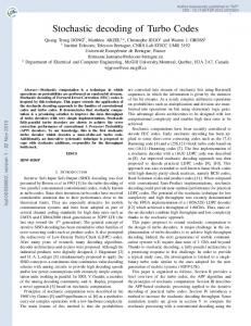
MLSDA, however, genuinely redirects and merges any two paths that share a common node, resulting in a stack without coexistence of crossed paths. A remarkable feature of the new ML path metric is that when a newly extended path merges with an existing path of longer length, the ML path metric of the newly extended path is always greater than or equal to the cumulative ML metric of the existing path up to the merged node. Therefore, a newly generated path that is shorter than its merged path can be immediately deleted, reducing the redirection overhead of the MLSDA only to the case in which the newly generated path and the merged existing path are equally long.11 That is, they merged at their end node. In such case, the redirection is merely a deletion of the path with larger path metric. Figures 11–12 show the performances of the MLSDA for (2, 1, 6) and (2, 1, 16) convolutional codes transmitted over the AWGN channel. Specifically, Fig. 11 compares the bit error rate (BER) of the MLSDA with those obtained by the Viterbi and the stack algorithms. Both the MLSDA and the Viterbi algorithm yield the same BER since they are both maximum-likelihood decoders. Figure 11 also shows that the MLSDA provides around 1.5 dB advantage over the stack algorithm at BER=10−5 , when both algorithms 11
Notably, for the new ML path metric, the path that survives is always the one with smaller path metric,
contrary to the sequential decoding algorithm in terms of the Fano metric, in which the path with larger Fano metric survives.
37
employ the same input sequence of length 40. Even when the length of the input sequence of the stack algorithm is extended to 200, the MLSDA with input sequence of length 40 still offers an advantage of about 0.5 dB at BER= 10−6 . Figure 12 collects the empirical results concerning the MLSDA with an input sequence of length 40 for (2, 1, 6) code, and the stack algorithm with input sequences of lengths 100 and 200 for (2, 1, 16) code. The three curves indicate that the MLSDA with an input sequence of smaller length 40 for (2, 1, 6) code provides an advantage of 1.0 dB over the stack algorithm with much longer input sequences and larger constraint length at BER=10−6 . The above simulations lead to the conclusion that the stack algorithm normally requires a sufficiently long input sequence to converge to a low BER, which necessarily results in a long decoding delay and high demand for stack space. By adopting a new sequential decoding metric, the MLSDA can achieve the same performance using a much shorter input sequence; hence, the decoding delay and the demand for stack space can be significantly reduced. Furthermore, unlike the Fano metric, the new ML metric adopted in the MLSDA does not depend on the knowledge of the channel, such as SNR, for codes transmitted over the AWGN channel. Consequently, the MLSDA and the Viterbi algorithm share a common nature that their performance is insensitive to the accuracy of the channel SNR estimate for AWGN channels. IX. Performance characteristics of sequential decoding An important feature of sequential decoding is that the decoding time varies with the received vector, because the number of paths examined during the decoding process differs for different received vectors. The received vector in turn varies according to the noise statistics. The decoding complexity can therefore be legitimately viewed as a random variable whose probability distribution is defined by the statistics of the received vector. The statistics of sequential decoding complexity have been extensively investigated using the random coding technique [40, 41, 15, 42, 43, 36, 44]. Instead of analyzing the complexity distribution with respect to a specific deterministic code, the average complexity distribution for a random code was analyzed. In practical applications, the
38
1 10−1 10−2
b cs
?
c bs
?
10−3
MLSDA and VA with input sequence of length 40 Stack algorithm with input sequence of length 40 MLSDA and VA with input sequence of length 200 Stack algorithm with input sequence of length 200
c bs
?
BER 10−4
c sb
?
10−5 10−6
c b s
1
2
3
4
b
?
c
?
b
5
6
10−7
s c
7
Eb /N0 in dB Fig. 11. Bit error rates (BER) of the MLSDA, the Viterbi algorithm (VA), and the stack algorithm for binary (2, 1, 6) convolutional code with generators g1 = 634 (octal), g2 = 564 (octal), and input sequences of lengths 40 and 200. [Source: Fig. 1 in [38]]
convolutional codes are always deterministic in their generator polynomials. Nevertheless, taking the aspect of a random convolutional code, in which the coefficients of the generator polynomials are random, facilitates the analysis of sequential decoding complexity. The resultant average decoding complexity (where the decoding complexity is directly averaged over all possible generator polynomials) can nonetheless serve as a quantitative guide to the decoding complexity of a practical deterministic code. In analyzing the average decoding complexity, a correct code path that corresponds to the transmitted codeword over the code tree or trellis always exists, even if the convolutional encoder is now random. Extra computation time is introduced, whenever the search process of the decoder deviates from the correct code path due to a noisedistorted received vector. The incorrect paths that deviate from the correct code path can be classified according to the first node at which the incorrect and the correct code paths depart from each other. Denote by Sj the subtree that contains all incorrect paths that branch from the jth node on the correct path, where 0 ≤ j ≤ L − 1 and L is the
39
1 10−1 10−2 10−3
BER
MLSDA and VA for (2, 1, 6) code with input sequence of length 40 Stack algorithm for (2, 1, 16) code with input sequence of length 100 Stack algorithm for (2, 1, 16) code with input sequence of length 200
s c b
s c b
10−4
cs b
10−5
s c b
c b
c b
s
10−6 10−7
2
2.5
3
3.5
4
4.5
5
5.5
6
Eb /N0 in dB Fig. 12. Bit error rates (BER) of the MLSDA and Viterbi algorithm for binary (2, 1, 6) convolutional code with generators g1 = 634 (octal), g2 = 564 (octal) and an input sequence of length 40. Also, BERs of the stack algorithm for binary (2, 1, 16) convolutional code with generators g 1 = 1632044, g2 = 1145734 and input sequences of lengths 100 and 200. [Source: Fig. 2 in [38]]
length of the code input sequences. Then, an upper probability bound12 on the average computational complexity Cj defined as the number of branch metric computations due to the examination of those incorrect paths in Sj can be established as Pr {Cj ≥ N } ≤ AN −ρ
(10)
for some 0 < ρ < ∞ and any 0 ≤ j ≤ L − 1, where A is a constant that varies for different sequential decoding algorithms. The bound is independent of j because, during its derivation, L is taken to infinity such that all incorrect subtrees become identical in principle. The distribution characterized by the right-hand-side of (10) is a Pareto distribution, and ρ is therefore named the Pareto exponent. Experimental studies indicate that the constant A usually lies between 1 and 10 [1]. The Pareto exponent ρ is uniquely 12
The bound in (10) was first established by Savage for random tree codes for some integer value of ρ [41], where
random tree codes constitute a super set of convolutional codes. Later, Jelinek [43] extended its validity for random tree codes to real-valued ρ ≥ 1, satisfying (11). The validity of (10) for random convolutional codes was substantiated by Falconer [42] for 0 < ρ < 1, and by Hashimoto and Arimoto [44] for ρ ≥ 1.
40
determined by the code rate R using the formula R=
E0 (ρ) ρ
(11)
for 0 < R < C, where E0 (ρ) is the Gallager function [45, Eq. (5.6.14)] and C is the channel capacity (cf. footnote 7). For example, the Gallager function and the channel capacity for the binary symmetric channel with crossover probability p are respectively given by ¤ £ E0 (ρ) = ρ − (1 + ρ) log2 p1/(1+ρ) + (1 − p)1/(1+ρ) ,
(12)
and C = 1 + p log2 (p) + (1 − p) log2 (1 − p). Equations (11) and (12) together imply that ρ goes to infinity as R ↓ 0, and ρ approaches zero when R ↑ C.
Figure 13 gives the Pareto exponents for code rates
R = 1/4, 1/3, 1/2, 2/3, 3/4. 6.5 6 5.5 5 4.5 4 ρ 3.5 3 2.5 2 1.5 1 0.5
R = 1/4 R = 1/3 R = 1/2 R = 2/3 R = 3/4
4
5
6 7 8 Eb /N0 in dB
9
10
Fig. 13. Pareto exponent as a function of Eb /N0 for a BSC with crossover probability p = p √ R∞ (1/2)erfc( Eb /N0 ), where erfc(x) = (2/ π) x exp{−x2 }dx is the complementary error function.
A converse argument to (10), due to Jacobs and Berlekamp [15], states that no sequential decoding algorithm can achieve a computational distribution better than the
41
Pareto distribution of (10), given that no decoding error results for convolutional codes. Specifically, they showed that for a Pareto exponent that satisfies (11), Pr { Cj ≥ N | correct decoding} > [1 − o(N )]N −ρ ,
(13)
where o(·) is the little-o function, satisfying o(x) → 0 as x → ∞. The two bounds in (10) and (13) coincide only when N is sufficiently large. Based on multiple branching process technique [46], close-form expressions of the average computational complexity of sequential decoding were derived in [47, 48, 49]. However, these close-form expressions were only suited for small N . Inequalities (10) and (13) also show that the two bounds are independent of the code constraint length. This observation confirms the claim made in the Introduction that the average computational effort for sequential decoding is in principle independent of the code constraint length. Inequalities (10), (13) and the observation that Cj ≥ 1 jointly yield Z ∞ Z ∞ E[Cj ] = Pr{Cj ≥ N }dN ≤ AN −ρ dN , 1
1
and E[Cj |correct decoding] = ≥
∞
Z
Z1 ∞ 1
Pr { Cj ≥ N | correct decoding} dN [1 − o(N )]N −ρ dN .
Therefore, if the Pareto exponent ρ is greater than unity, E[Cj ] is bounded from above. Conversely, if E[Cj |correct decoding] < ∞, then ρ > 1. Since the probability of correct decoding is very close to unity in most cases of interest, ρ > 1 is widely accepted as a sufficient and necessary condition for E[Cj ] to be bounded. This result gives rise to the term, computational cutoff rate R0 = E0 (1), for sequential decoding. From (11), ρ > 1 if, and only if, R < R0 = E0 (1), meaning that the cutoff rate R0 is the largest code rate under which the average complexity of sequential decoding is finite. Thus, sequential decoding becomes computationally implausible once the code rate exceeds the cutoff rate R0 . This theoretical conclusion can be similarly observed from simulations.
42
Can the computational cutoff rate be improved? The question was answered by a proposal made by Flaconer [42], concerning the use of a hybrid coding scheme. The proposed communication system consists of an (nout , kout ) outer Reed-Solomon encoder, nout parallel (nin , 1, m) inner convolutional encoders, nout parallel noisy channels, nout sequential decoders for inner convolutional codes, and an algebraic decoder for the outer Reed-Solomon code. These five modules work together in the following fashion. The outer Reed-Solomon encoder encodes kout input symbols into nout output symbols, each of which is b bits long with the last m bits equal to zero. Then, each of the nout output symbols is fed into its respective binary (nin , 1, m) convolutional encoder in parallel, and induces nin × b output code bits. Thereafter, these nout (nin b)-bit streams are simultaneously transmitted over nout independent channels, where the nout independent channels may be created by time-multiplexing over a single channel. Upon receiving nout noisedistorted received vectors of dimension nin b, the nout sequential decoders reproduce the nout output symbols through a sequential codeword search. If any sequential codeword search is not finished before a pre-specified time, its output will be treated as an erasure. The final step is to use an algebraic Reed-Solomon decoder to regenerate the kout input symbols based upon the nout output symbols obtained from the nout parallel sequential decoders. The effective code rate of this hybrid system is Reffective =
kout (b − m) . nout nin b
The largest effective code rate under which the hybrid system is computationally practical has been proved to improve over E0 (1) [42]. Further improvement along the line of code concatenation can be found in [50, 51]. The basis of the performance analysis for the aforementioned sequential decoding is random coding, and has nothing to do with any specific properties of the applied code, except the code rate R. Zigangirov [34] proposed to analyze the statistics of Cj for deterministic convolutional codes with an infinite memory order (i.e., m = ∞) in terms of recursive equations, and determined that for codes transmitted over BSCs and decoded
43
by the tree-based stack algorithm, E[Cj ] ≤
ρ −(−nα+β)/(1+ρ)−k 2 ρ−1
(14)
for R < R0 = E0 (1), where ρ is the Pareto exponent that satisfies (11), and α and β are defined in the sentence following Eq. (4). Zigangirov’s result again suggested that E[C j ] is bounded for R < R0 , even when the deterministic convolutional codes are considered. A similar result was also established for the Fano algorithm in [34]. Another code-specific estimate of sequential decoding complexity was due to Chevillat and Costello [52, 53]. From simulations, they ingeniously deduced that the computational complexity of a sequential decoder is indeed related to the column distance function (CDF) of the applied code. They then established that for a convolutional code transmitted over a BSC with crossover probability p, Pr {Cj ≥ N } < A Nd exp {−λ1 dc (`) + λ2 `}
(15)
for R < 1 + 2p log2 (p) + (1 − 2p) log2 (1 − p), where A, λ1 and λ2 are factors determined by p and code rate R, Nd is the number of length-[n(` + 1)] paths with Hamming weight equal to dc (`), ` is the integer part of log2k N , and dc (r) is the CDF of the applied code. They concluded that a convolutional code with a rapidly increasing CDF can yield a markedly smaller sequential decoding complexity. The outstanding issue is thus how to construct similar convolutional codes for use in sequential decoding. The issue will be further explored in Section XI. Next, the upper bounds on the bit error rate of sequential decoding are introduced. Let PSj be the probability that a path belonging to the incorrect subtree Sj is decoded as the ultimate output. Then, [53] showed that for a specific convolutional code transmitted over a BSC with crossover probability p, PSj < B Nf exp {−γ dfree } ,
(16)
where B and γ are factors determined by p and code rate R, Nf is the number of code paths in Sj with Hamming weight equal to dfree , and dfree is the free distance of the applied code. The parameter γ is positive for all convolutional codes whose free distance
44
exceeds a lower limit determined by p and R. This result indicates that a small error probability for sequential decoding can be obtained by selecting a convolutional code with a large free distance and a small number of codewords with Hamming weight d free . The free distance of a convolutional code generally grows with its constraint length. The bit error rate can therefore be made desirably low when a convolutional code with a sufficiently large constraint length is employed, as the computational complexity of sequential decoding is independent of the code constraint length. However, when a code with a large constraint length is used, the length of the input sequences must also be extended such that the effective code rate kL/[n(L+m)] is closely approximated by code rate R = k/n. More discussion of the bit error rates of sequential decoding can be found in [40, 36, 54]. X. Buffer overflow and system considerations As already demonstrated by the hardware implementation of the Fano algorithm in Section VII, the input buffer at the decoder end for the temporary storage of the received vector is finite. The on-line decoder must therefore catch up to the input rate of the received vector such that the storage space for obsolete components of the received vector can be freed to store upcoming received components. Whenever an input buffer overflow is encountered, some of the still-in-use content in the input buffer must be forcefully written over by the new input, and the decoder must resynchronize to the new contents of the input buffer; hence, input erasure occurs. The overall codeword error P s of a sequential decoder thus becomes: Ps ' Pe + Perasure , where Pe is the undetected word error under the infinite input buffer assumption, and Perasure is the erasure probability. For a code with a long constraint length and a practically sized input buffer, Pe is markedly smaller than Perasure , so the overall word error is dominated by the probability of input buffer overflow. In this case, effort is reasonably focused on reducing Perasure . When the code constraint length is only moderately large, a tradeoff between Pe and Perasure must be made. For example, reducing the bucket spac-
45
ing for the stack-bucket-enabled stack algorithm or lowering the step size for the Fano algorithm results in a smaller Pe , but increases E[Cj ] and hence Perasure . The choice of path metrics, as indicated in Section V, also yields a similar tradeoff between P e and Perasure . Accordingly, a balance between these two error probabilities must be maintained in practical system design. The probability of buffer overflow can be analyzed as follows. Let B be the size of the input buffer measured in units of branches; hence, the input buffer can store nB bits for an (n, k, m) convolutional code. Also let 1/T (bits/second) be the input rate of the received vector. Suppose that the decoder can perform µ branch metric computations in n × T seconds. Then if over µB branch computations are performed for paths in the jth incorrect subtree, the jth received branch in the input buffer must be written over by the new received branch. To simplify the analysis, assume that the entire buffer is simply reset when a buffer overflow occurs. In other words, the decoder aborts the present codeword search, and immediately begins a new search according to the new received vector. From Eq. (10), the probability of performing more than µB branch computations for paths in Sj is upper-bounded by A(µB)−ρ . Hence, the erasure probability [41, 55] for input sequences of length L is upper-bounded by Perasure ≤ L A (µB)−ρ .
(17)
Taking L = 1000, A = 5, µ = 10, B = 105 and R = 1/2 yields ρ = 1.00457 and Perasure ≤ 4.694 × 10⁻³ . Three actions can be taken to avoid eliminating the entire received vector when the input buffer overflow occurs: (1) just inform the outer mechanism that an input erasure occurs, and let the outer mechanism take care of the decoding of the respective input sequences, (2) estimate the respective input sequences by a function mapping from the received vector to the input sequence, and (3) output the tentative decoding results yet obtained. The previous section already demonstrated an example of the first action using the hybrid coding system. The second action can be taken whenever an input sequence to a convolutional encoder can be recovered from its codewords through a function mapping. Two typical convolutional codes whose input sequence can be directly mapped from the
46
codewords are the systematic code and the quick-look-in code (to be introduced in the next section). A decoder can also choose to output a tentative decoded input sequence if the third action is taken. A specific example for the third action, named the multiple stack algorithm, is introduced in the next paragraph. In 1977, Chevillat and Costello [56] proposed a multiple stack algorithm (MSA), which eliminated entirely the possibility of erasure in the sense that the decoded output is always based upon the codeword search. The MSA, as its name implies, acts exactly like the stack algorithm except that it accommodates multiple stacks. During decoding, the MSA first behaves as the stack algorithm by using only its main stack of size zmain . When the main stack reaches its limit, the best t paths in the main stack are transferred to a smaller second stack with size z ¿ zmain . Then the decoding process proceeds just like the stack algorithm, but now using the second stack. If a path reaches the end of the search tree before the second stack is filled, then the path is stored as a tentative decision, and the second stack is eliminated. The MSA then returns to the main stack that has t vacancy spaces for new paths because the top t paths have been removed. If another path reaches the end of the search tree before the main stack is filled up again, the decoder compares its path metric with that of the current tentative decision, and outputs the one with larger metric, and stops. Now in case the second stack is filled up before a code path is located, then a third stack with the same size z is created such that the top t paths in the second stack are transferred to it. The codeword search process then proceeds over the third stack until either a tentative decision can be made or a new stack needs to be created. Additional stacks of size z are formed whenever necessary. The decoder always compares the newly located code path with the previous tentative decision, and retains the better one. With some properly selected system parameters including zmain , z, t, and input buffer size, the MSA guarantees that whenever an input erasure occurs, a tentative decision is always ready for output [56]. Simulation results show that even though the stack maintenance of the MSA is more complex than the stack algorithm, the bit error rate of the former is much lower than that of the latter (cf. Fig. 14). Further improvements of the MSA can be found in [57, 58].
47
0.1
(2, 1, 7) code (2, 1, 14) code
0.01 0.001 0.0001 BER 1e-05 1e-06 1e-07 1e-08
4
4.5
5
5.5 6 Eb /N0 in dB
6.5
7
Fig. 14. The MSA bit error rates (BER) for (2, 1, 7) and (2, 1, 14) convolutional codes with an input sequence of length 64. The system parameters for (2, 1, 7) and (2, 1, 14) convolutional codes are (zmain , z, t) = (1024, 11, 3) and (zmain , z, t) = (2900, 11, 3), respectively. The input erasure is emulated by an upper limit on branch metric computations Clim , which is 1700 and 3300 for (2, 1, 7) and (2, 1, 14) convolutional codes, respectively. [Reproduced in part from Fig. 3 in [57].]
XI. Code construction for sequential decoding A rapid column distance growth in CDF has been conjectured to help the early rejection of incorrect paths for sequential decoding algorithms [59]; this conjecture was later substantiated by Chevillat and Costello both empirically [52] and analytically [53]. In an effort to construct a good convolutional code for sequential decoding, Johannesson proposed [60] that the code distance profile, defined as {dc (1), dc (2), . . . , dc (m + 1)}, can be used, instead of the entire code distance function dc (·), as a “criterion” for good code construction. His suggestion greatly reduced the number of possible code designs that must be investigated. A code C is said to have a better distance profile than another code C 0 with the same
code rate and memory order, if there exists ` with 1 ≤ ` ≤ m + 1 such that dc (j) = d0c (j)
for 1 ≤ j ≤ ` − 1 and dc (`) > d0c (`), where dc (·) and d0c (·) are the CDFs of codes C and C 0 , respectively. In other words, a code with a better distance profile exhibits a faster
48
initial column distance growth in its CDF. A code is said to have an optimal distance profile, and is called an ODP code, if its distance profile is superior to that of any other code with the same code rate and memory order. The searching of ODP codes was extensively studied by Johannesson and Passke [60, 61, 62, 63]. They found that the ODP condition could be imposed on a half-rate (R = 1/2) short constraint length code without penalty in the code free distance [60]. That is, the half-rate ODP code with a short constraint length can also be the code with the largest free distance of all codes with the same code rate and memory order. Tables I and II list the half-rate ODP codes for systematic codes and nonsystematic codes, respectively. Comprehensive information on ODP codes can be found in [34]. These tables notably reveal that the free distance of a systematic ODP code is always inferior to that of a nonsystematic ODP code with the same memory order. Employing ODP codes, while notably reduces the number of metric computations for sequential decoding, does not ensure erasure-free performance in practical implementation. If an erasure-free sequential decoding algorithm such as the MSA cannot be adopted due to certain practical considerations, the decoder must still force an immediate decision by just taking a quick look at the received vector, once input erasure occurs. This seems to suggest that a systematic ODP code is preferred, even if it has a smaller free distance than its non-systematic ODP counterpart. In such case, the deficiency on the free distance of the systematic ODP codes can be compensated for by selecting a larger memory order m. However, when a convolutional code with large m is used, the length of the input sequences must be proportionally extended, otherwise the effective code rate cannot be well-approximated by the convolutional code rate, and the performance to some extent degrades. This effect motivates the attempt to construct a class of non-systematic ODP codes with the “quick-look” property and a free distance superior to that of systematic codes. Such a class of non-systematic codes has been developed by Massey and Costello, called the quick-look-in (QLI) convolutional codes [59]. The generator polynomials of these half-rate QLI convolutional codes differ only in the second coefficient. Specifically,
49
TABLE I List of R = 1/2 systematic codes with optimal distance profile [34].
m
g2
dfree
1
6
3
2
7
4
3
64
4
4
66
5
5
73
6
6
674
6
7
714
6
8
671
7
9
7154
8
10
7152
8
11
7153
9
12
67114
9
13
67116
10
14
71447
10
15
671174
10
16
671166
12
17
671166
12
18
6711454
12
19
7144616
12
20
7144761
12
21
71447614
12
22
71446166
14
23
67115143
14
24
714461654
15
25
671145536
15
26
714476053
16
27
7144760524
16
28
7144616566
16
29
7144760535
18
30
67114543064
16
31
67114543066
18
50
TABLE II List of R = 1/2 nonsystematic codes with optimal distance profile [34].
m
g1
g2
dfree
1
6
4
3
2
7
5
5
3
74
54
6
4
62
56
7
5
77
45
8
6
634
564
10
7
626
572
10
8
751
557
12
9
7664
5714
12
10
7512
5562
14
11
6643
5175
14
12
63374
47244
15
13
45332
77136
16
14
65231
43677
17
15
727144
424374
18
16
717066
522702
19
17
745705
546153
20
18
6302164
5634554
21
19
5122642
7315626
22
20
7375407
4313045
22
21
67520654
50371444
24
22
64553062
42533736
24
23
55076157
75501351
26
24
744537344
472606614
26
25
665041116
516260772
27
51
their generator polynomials satisfy g1 (x) = g2 (x) + x, where addition of coefficients is based on modulo-2 operation, allowing the decoder to recover the input sequence u(x) by summing the two output sequences v 1 (x) and v 2 (x) as x · u(x) = v 1 (x) + v 2 (x).
(18)
If p is the individual bit error probability in the codeword v, then the bit error probability due to recovering information sequence u from v through (18) is shown to be approximately 2p [59]. Table III gives a list of QLI ODP convolutional codes [34]. XII. Conclusions Although sequential decoding has a longer history than maximum-likelihood decoding based on the Viterbi algorithm, its practical applications are not as popular, because the highly repetitive “pipeline” nature of the Viterbi decoder makes it very suitable for hardware implementation. Furthermore, a sequential decoder usually requires a longer decoding delay (defined as the time between the receipt of a received branch and the output of its respective decoding decision) than a Viterbi decoder. Generally, the decoding delay of a sequential decoder for an (n, k, m) convolutional code is around n × B, where B is the number of received branches that an input buffer can accommodate. Yet, the decoding delay of a Viterbi decoder can be made a small multiple, often ranging from 5 to 10, of n × m. On the other hand, references [64] and [65] showed that sequential decoding is highly sensitive to the channel parameters such as an inaccurate estimate of channel SNR and an incomplete compensation of phase noise. The Viterbi algorithm, however, was proven to be robust for imperfect channel identification, again securing the superiority of the Viterbi decoder in practical applications. Nevertheless, there are certain situations that the sequential decoding fits well, especially in decoding convolutional codes having a large constraint length. In addition, the sequential decoder can send a timely retransmission request by detecting the occurrence of an input buffer overflow [66]. Very recently, sequential decoding has attracted some attention in the field of mobile communications [67] in which a demand of low bit error rate is required. Such applications are beyond the scope of this article, and interested
52
TABLE III List of R = 1/2 QLI codes with optimal distance profile [34].
m
g1
df ree
2
7
5
3
74
6
4
76
6
5
75
8
6
714
8
7
742
9
8
743
9
9
7434
10
10
7422
11
11
7435
12
12
74044
11
13
74046
13
14
74047
14
15
740464
14
16
740462
15
17
740463
16
18
7404634
16
19
7404242
15
20
7404155
18
21
74041544
18
22
74042436
19
23
74041567
19
24
740415664
20
25
740424366
20
26
740424175
22
27
7404155634
22
28
7404241726
23
29
7404154035
24
30
74041567514
23
31
74041567512
25
53
readers can refer to [1, 68, 69]. Acknowledgement Prof. Marc P. C. Fossorier of University of Hawaii and Prof. John G. Proakis are appreciated for their careful reviews and valuable comments. Mr. Tsung-Ju Wu and Mr. Tsung-Chi Lin are also appreciated for preparing the figures and checking the examples in this manuscript. References [1]
S. Lin and D. J. Costello, Jr., Error Control Coding: Fundamentals and Applications, Englewood Cliffs,
[2]
J. M. Wozencraft, “Sequential decoding for reliable communications,” IRE Nat. Conv. Rec., vol. 5, pt. 2,
NJ: Prentice-Hall, Inc., 1983. pp. 11–25, 1957. [3]
J. M. Wozencraft and B. Reiffen, Sequential Decoding, Cambridge, Mass: MIT Press, 1961.
[4]
R. M. Fano, “A heuristic discussion of probabilistic decoding,” IEEE Trans. Inform. Theory, vol. IT-9, no. 2, pp. 64–73, April 1963.
[5]
K. Sh. Zigangirov, “Some sequential decoding procedures,” Probl. Peredachi Inf., 2, pp. 13–25, 1966.
[6]
F. Jelinek, “A fast sequential decoding algorithm using a stack,” IBM J. Res. and Dev., 13, pp. 675–685,
[7]
N. J. Nilsson, Principle of Artificial Intelligence, Palo Alto, CA: Tioga Publishing Co., 1980.
[8]
S. B. Wicker, Error Control Systems for Digital Communication and Storage, Englewood Cliffs, NJ:
[9]
A. J. Viterbi, “Error bound for convolutional codes and an asymptotically optimum decoding algorithm,”
November 1969.
Prentice-Hall, Inc., 1995. IEEE Trans. Inform. Theory, vol. IT-13, no. 2, pp. 260–269, April 1967. [10] J. L. Massey, Threshold Decoding, MIT Press, Cambridge, Mass., 1963. [11] G. D. Forney, Jr., “Review of random tree codes,” Appendix A. Study of Coding Systems Design for Advanced Solar Missions. NASA Contract NAS2-3637. Codex Corporation. December 1967. [12] J. Pearl, Heuristics: Intelligent Search Strategies for Computer Problem Solving, Reading, MA: AddisonWesley Publishing Company, 1984. [13] Y. S. Han, C. R. P. Hartmann, and C.-C. Chen, “Efficient priority-first search maximum-likelihood softdecision decoding of linear block codes,” IEEE Trans. Inform. Theory, vol. 39, no. 5, pp. 1514–1523, September 1993. [14] Y. S. Han, “A new treatment of priority-first search maximum-likelihood soft-decision decoding of linear block codes,” IEEE Trans. Inform. Theory, vol. 44, no. 7, pp. 3091–3096, November 1998. [15] I. M. Jacobs and E. R. Berlekamp, “A lower bound to the distribution of computation for sequential decoding,” IEEE Trans. Inform. Theory, vol. IT-13, no. 2, pp. 167–174, April 1967. [16] T. M. Cover and J. A. Thomas, Elements of Information Theory, New York, NY: John Wiley and Sons, 1991.
54
[17] J. L. Massey, “Variable-length codes and the fano metric,” IEEE Trans. Inform. Theory, vol. IT-18, no. 1, pp. 196–198, January 1972. [18] E. A. Bucher, “Sequential decoding of systematic and nonsystematic convolutional codes with arbitrary decoder bias,” IEEE Trans. Inform. Theory, vol. IT-16, no. 5, pp. 611–624, September 1970. [19] F. Jelinek, “Upper bound on sequential decoding performance parameters,” IEEE Trans. Inform. Theory, vol. IT-20, no. 2, pp. 227–239, March 1974. [20] Y. S. Han, P.-N. Chen, and M. P. C. Fossorier, “A generalization of the fano metric and its effect on sequential decoding using a stack,” in IEEE Int. Symp. on Information Theory, Lausanne, Switzerland, 2002. [21] K. Sh. Zigangirov, private communication, February, 2002. [22] J. M. Geist, “Am empirical comparison of two sequential decoding algorithms,” IEEE Trans. Commun. Technol., vol. COM-19, no. 4, pp. 415–419, August 1971. [23] D. Haccoun and M. J. Ferguson, “Generalized stack algorithms for decoding convolutional codes,” IEEE Trans. Inform. Theory, vol. IT-21, no. 6, pp. 638–651, November 1975. [24] J. B. Anderson and S. Mohan, “Sequential coding algorithms: a survey and cost analysis,” IEEE Trans. Commun., vol. COM-32, no. 2, pp. 169–176, February 1984. [25] S. Mohan and J. B. Anderson, “Computationally optimal metric-first code tree search algorithms,” IEEE Trans. Commun., vol. COM-32, no. 6, pp. 710–717, June 1984. [26] D. E. Knuth, The Art of Computer Programming. Volume III: Sorting and Searching, Reading, MA: Addison-Wesley, 1973. [27] P. Lavoie, D. Haccoun, and Y. Savaria, “A systolic architecture for fast stack sequential decoders,” IEEE Trans. Commun., vol. 42, no. 5, pp. 324–335, May 1994. [28] S. Kallel and K. Li, “Bidirectional sequential decoding,” IEEE Trans. Inform. Theory, vol. 43, no. 4, pp. 1319–1326, July 1997. [29] J. M. Geist, “Search properties of some sequential decoding algorithms,” IEEE Trans. Inform. Theory, vol. IT-19, no. 4, pp. 519–526, July 1973. [30] Jr. G. D. Forney and E. K. Bower, “A high-speed sequential decoder: prototype design and test,” IEEE Trans. Commun. Technol., vol. COM-19, no. 5, pp. 821–835, October 1971. [31] I. M. Jacobs, “Sequential decoding for efficient communication from deep space,” IEEE Trans. Commun. Technol., vol. COM-15, no. 4, pp. 492–501, August 1967. [32] J. W. Layland and W. A. Lushbaugh, “A flexible high-speed sequential decoder for deep space channels,” IEEE Trans. Commun. Technol., vol. COM-19, no. 5, pp. 813–820, October 1978. [33] M. Shimada, T. Todoroki, and K. Nakamura, “Development of variable-rate sequential decoder LSI,” in IEEE International Conference on Communications, 1989, pp. 1241–1245. [34] R. Johannesson and K. Sh. Zigangirov, Fundamentals of Convolutional Coding, IEEE Press: Piscataway, NJ, 1999. [35] J. Geist, Algorithmic aspects of sequential decoding, Ph.D. thesis, Dep. Elec. Eng., Univ. Notre Dame, Notre Dame, Ind., 1970. [36] G. D. Forney, Jr., “Convolutional codes III: Sequential decoding,” Inf. Control, 25, pp. 267–269, July 1974. [37] N. B´elanger, D. Haccoun, and Y. Savaria, “A multiprocessor architecture for multiple path stack sequential decoders,” IEEE Trans. Commun., vol. 42, no. 2/3/4, pp. 951–957, February/March/April 1994.
55
[38] Y. S. Han, P.-N. Chen, and H.-B. Wu, “A maximum-likelihood soft-decision sequential decoding algorithm for binary convolutional codes,” IEEE Trans. Commun., vol. 50, no. 2, pp. 173–178, February 2002. [39] J. Snyders and Y. Be’ery, “Maximum likelihood soft decoding of binary block codes and decoders for the golay codes,” IEEE Trans. Inform. Theory, pp. 963–975, September 1989. [40] H. L. Yudkin, Channel state testing in information decoding, Ph.D. thesis, MIT, Cambridge, Mass, 1964. [41] J. E. Savage, “Sequential decoding-the computation problem,” Bell Sys. Tech. J., vol. 45, pp. 149–175, January 1966. [42] D. D. Falconer, “A hybrid decoding scheme for discrete memoryless channels,” Bell Syst. Tech. J., vol. 48, pp. 691–728, March 1969. [43] F. Jelinek, “An upper bound on moments of sequential decoding effort,” IEEE Trans. Inform. Theory, vol. IT-15, no. 1, pp. 140–149, January 1969. [44] T. Hashimoto and S. Arimoto, “computational moments for sequential decoding of convolutional codes,” IEEE Trans. Inform. Theory, vol. IT-25, no. 5, pp. 584–591, 1979. [45] R. G. Gallager, Information Theory and Reliable Communication, New York, NY: John Wiley and Sons, 1968. [46] W. Feller, An Introduction to Probability Theory and its Applications, New York, NY: John Wiley and Sons, 1970. [47] R. Johannesson, “On the distribution of computation for sequential decoding using the stack algorithm,” IEEE Trans. Inform. Theory, vol. IT-25, no. 3, pp. 323–332, May 1979. [48] D. Haccoun, “A branching process analysis of the average number of computations of the stack algorithm,” IEEE Trans. Inform. Theory, vol. IT-30, no. 3, pp. 497–508, May 1984. [49] R. Johannesson and K. Sh. Zigangirov, “On the distribution of the number of computations in any finite number of subtrees for the stack algorithm,” IEEE Trans. Inform. Theory, vol. IT-31, no. 1, pp. 100–102, January 1985. [50] F. Jelinek and J. Cocke, “Bootstrap hybrid decoding for symmetrical binary input channel,” Inf. Control, 18, pp. 261–298, April 1971. [51] O. R. Jensen and E. Paaske, “Forced sequence sequential decoding: a concatenated coding system with iterated sequential inner decoding,” IEEE Trans. Commun., vol. 46, no. 10, pp. 1280–1291, October 1998. [52] P. R. Chevillat and D. J. Costello, Jr., “Distance and computation in sequential decoding,” IEEE Trans. Commun., vol. COM-24, no. 4, pp. 440–447, April 1978. [53] P. R. Chevillat and D. J. Costello, Jr., “An analysis of sequential decoding for specific time-invariant convolutional codes,” IEEE Trans. Inform. Theory, vol. IT-24, no. 4, pp. 443–451, July 1978. [54] A. J. Viterbi and J. K. Omura, Principles of Digital Communication and Coding, New York, NY: McGrawHill Book Company, 1979. [55] J. E. Savage, “The distribution of the sequential decoding computation time,” IEEE Trans. Inform. Theory, vol. IT-12, no. 2, pp. 143–147, April 1966. [56] P. R. Chevillat and D. J. Costello, Jr., “A multiple stack algorithm for erasurefree decoding of convolutional codes,” IEEE Trans. Commun., vol. COM-25, no. 12, pp. 1460–1470, December 1977. [57] H. H. Ma, “The multiple stack algorithm implemented on a zilog z-80 microcomputer,” IEEE Trans. Commun., vol. COM-28, no. 11, pp. 1876–1882, November 1980.
56
[58] K. Li and S. Kallel, “A bidirectional multiple stack algorithm,” IEEE Trans. Commun., vol. 47, no. 1, pp. 6–9, January 1999. [59] J. L. Massey and Jr. D. J. Costello, “Nonsystematic convolutional codes for sequential decoding in space applications,” IEEE Trans. Commun. Technol., vol. COM-19, no. 5, pp. 806–813, October 1971. [60] R. Johannesson, “Robustly optimal rate one-half binary convolutional codes,” IEEE Trans. Inform. Theory, vol. IT-21, no. 4, pp. 464–468, July 1975. [61] R. Johannesson, “Some long rate one-half binary convolutional codes with an optimal distance profile,” IEEE Trans. Inform. Theory, vol. IT-22, no. 5, pp. 629–631, September 1976. [62] R. Johannesson, “Some rate 1/3 and 1/4 binary convolutional codes with an optimal distance profile,” IEEE Trans. Inform. Theory, vol. IT-23, no. 2, pp. 281–283, March 1977. [63] R. Johannesson and E. Paaske, “Further results on binary convolutional codes with an optimal distance profile,” IEEE Trans. Inform. Theory, vol. IT-24, no. 2, pp. 264–268, March 1978. [64] J. A. Heller and I. W. Jacobs, “Viterbi decoding for satellite and space communication,” IEEE Trans. Commun. Technol., vol. COM-19, no. 5, pp. 835–848, October 1971. [65] I. M. Jacobs, “Practical applications of coding,” IEEE Trans. Inform. Theory, vol. IT-20, no. 3, pp. 305–310, May 1974. [66] A. Drukarev and Jr. D. J. Costello, “Hybrid ARQ error control using sequential decoding,” IEEE Trans. Inform. Theory, vol. IT-29, no. 4, pp. 521–535, July 1983. [67] P. Orten and A. Svensson, “Sequential decoding in future mobile communications,” in Proc. PIMRC ’97, 1997, vol. 3, pp. 1186–1190. [68] S. Kallel, “Sequential decoding with an efficient incremental redundancy ARQ strategy,” IEEE Trans. Commun., vol. 40, no. 10, pp. 1588–1593, October 1992. [69] P. Orten, “Sequential decoding of tailbiting convolutional codes for hybrid ARQ on wireless channels,” in Proc. IEEE Vehicular Technology Conference, 1999, vol. 1, pp. 279–284.