Efficient Decomposition of Polygons into L-Shapes with Applications to VLSI Layouts MARIO A. LOPEZ University of Denver and DINESH P. MEHTA University of Tennessee Space Institute
We present two practical algorithms for partitioning circuit components represented by rectilinear polygons so that they can be stored using the L-shaped corner stitching data structure; that is, our algorithms decompose a simple polygon into a set of nonoverlapping L-shapes and rectangles by using horizontal cuts only. The more general of our algorithms computes an optimal configuration for a wide variety of optimization functions, whereas the other computes a minimum configuration of rectangles and L-shapes. Both algorithms run in O(n 1 h log h) time, where n is the number of vertices in the polygon and h is the number of H-pairs. Because for VLSI data h is small, in practice these algorithms are linear in n. Experimental results on actual VLSI data compare our algorithms and demonstrate the gains in performance for corner stitching (as measured by different objective functions) obtained by using them instead of more traditional rectangular partitioning algorithms. Categories and Subject Descriptors: B.7.2 [Integrated Circuits]: Design Aids—layout; F.2.2 [Analysis of Algorithms and Problem Complexity]: Nonnumerical Algorithms and Problems—geometrical problems and computations; G.2.2 [Discrete Mathematics]: Graph Theory—graph algorithms General Terms: Algorithms Additional Key Words and Phrases: Corner stitching, L-shapes, partition, rectangle, rectilinear polygons
1. INTRODUCTION The corner stitching data structure was proposed by Ousterhout [1984] to store rectangular circuit components in the MAGIC system [Ousterhout et Authors’ addresses: M. A. Lopez, Department of Mathematics and Computer Science, University of Denver, Denver, CO 80208; email:
[email protected]; D.P. Mehta, Department of Computer Science, M.S. 21, University of Tennessee Space Institute, Tullahoma, TN 373888897; email:
[email protected]. Permission to make digital / hard copy of part or all of this work for personal or classroom use is granted without fee provided that the copies are not made or distributed for profit or commercial advantage, the copyright notice, the title of the publication, and its date appear, and notice is given that copying is by permission of the ACM, Inc. To copy otherwise, to republish, to post on servers, or to redistribute to lists, requires prior specific permission and / or a fee. © 1996 ACM 1084-4309/96/0700 –0371 $03.50 ACM Transactions on Design Automation of Electronic Systems, Vol. 1, No. 3, July 1996, Pages 371–395.
372
•
M. A. Lopez and D. P. Mehta
al. 1984]. It was subsequently extended to handle trapezoidal tiles in TAILOR [Marple et al. 1990], curved tiles [Se´quin and Fac¸anha 1993], and L-shaped tiles [Blust and Mehta 1993]. The corner stitching data structure is also discussed in Sherwani [1995]. Because, in practice, circuit components can be arbitrary rectilinear polygons, it is necessary to partition them into rectangles to enable them to be stored in the corner stitching format. MAGIC handles this by using horizontal lines to partition the polygons. This is not necessary from a theoretical standpoint, but it simplifies the implementation of the various corner stitching operations. Nahar and Sahni [1988] studied this problem and presented an O(n 1 k v log k v ) algorithm to decompose a polygon with n vertices and k v vertical inversions into rectangles using horizontal cuts only. (The number of vertical inversions of a polygon is defined as the minimum number of changes in vertical direction during a walk around the polygon divided by two.) The quantity k v was observed to be small for polygons encountered in VLSI mask data. Consequently, the Nahar-Sahni algorithm outperforms an O(n log n) planesweep algorithm on VLSI mask data. We note that this problem is different from the problem of decomposing a rectilinear polygon into a minimum number of rectangles using both horizontal and vertical cuts, which has been studied extensively in the literature.1 In the extension to corner stitching proposed by Blust and Mehta [1993], the data structure stores L-shaped tiles (hexagons) in addition to rectangular tiles. This L-shaped variant of corner stitching was motivated by a need for a data structure that could store rectilinear shapes more general than rectangles [Shanbhag et al. 1994; Mehta et al. 1995]. L-shaped objects, in particular, have been studied in the context of floorplanning [Wang and Wong 1990; Yeap and Sarrafzadeh 1993] and routing [Dai et al. 1985; Cai and Wong 1993]. Once again, because circuit components can be rectilinear polygons that are not rectangles or L-shapes, these components need to be partitioned in order to store them in the L-shaped corner stitching data structure. Furthermore, using horizontal cuts for partitioning is desirable inasmuch as it simplifies the implementation of the operations (which are now more complex than for the rectangular corner stitching data structure). This motivates the need for a fast and practical algorithm for partitioning polygons into L-shapes and rectangles using horizontal cuts only. In this paper, we present two algorithms to partition a rectilinear polygon into rectangles and L-shapes using only horizontal cuts. Both algorithms require O(n 1 h log h) time, where h 5 k v 2 1 denotes the number of H-pairs in the polygon, which we will define later. It is possible to improve the asymptotic time of both algorithms to O(n), by utilizing Chazelle’s [1991] O(n) triangulation algorithm in Step 1 of both of our algorithms (see Section 3). However, because for VLSI data h is small, using the procedure discussed in Section 3.1 results in fast algorithms that 1
Please see Ohtsuki [1982], Imai and Asano [1986], Liou et al. [1989], and Wu and Sahni [1991].
ACM Transactions on Design Automation of Electronic Systems, Vol. 1, No. 3, July 1996.
Decompositions of Polygons into L-Shapes
Fig. 1.
•
373
L-shaped tiles.
are more practical than an asymptotically optimal solution based on the significantly more difficult procedure proposed by Chazelle. Our first algorithm DP uses dynamic programming to obtain an optimal cost partition. Each tile has a cost associated with it and the cost of the partition is the sum of the costs of the tiles used in the partition. We assume the existence of an arbitrary function to compute the cost of a tile in constant time. The exact nature of this function depends on what we want to optimize. For example, to minimize the amount of storage required by the corner stitching data structure, the cost of a tile would be the number of bytes required to store that tile. In corner stitching, this quantity is determined by the tile orientation. Figure 1 shows the four possible types of L-shapes. These shapes are numbered according to the quadrant missing from the bounding rectangle of the L-shape. For instance, in Figure 1(a), the first quadrant is missing, so the L-shape type is L 1 . The tile cost is 36 bytes for each L 1 , L 2 , or L 4 shape used in the data structure, 44 bytes for each L 3 shape, and 28 bytes for each rectangle [Blust and Mehta 1993]. We refer to this version of DP as DP bytes . Another objective might be to minimize the number of tiles in the corner stitching data structure because the time required by corner stitching operations is related to the number of tiles in the data structure. In this case, each tile would have a cost of one unit. We refer to this version of DP as DP min . Alternatively, the designer might wish to minimize total cut length of the partition. The problem of minimizing total cut length was introduced by Lingas et al. [1982] in the context of partitioning a rectilinear polygon into rectangles. It was found that such a partition yields a good decomposition of the routing area into rectangular channels. An O(n 4 ) time algorithm was presented for rectilinear polygons without holes and the problem was shown to be NP-complete for rectilinear polygons with holes. Heuristics and approximation algorithms for the latter problem have been studied in the ACM Transactions on Design Automation of Electronic Systems, Vol. 1, No. 3, July 1996.
374
•
M. A. Lopez and D. P. Mehta
Fig. 2.
Partitioning a rectilinear polygon.
literature.2 The analogous problem for partitions into L-shapes and rectangles is motivated by Dai et al. [1985] and Cai and Wong [1993], wherein L-shaped channels have been considered as a means to eliminating cyclic precedence constraints in nonslicing floorplans. In this case, the cost of a tile is defined as the length of the cut (if any) that is used to form its lower boundary. We refer to this version of DP as DP cut . The requirement that an optimal partition be computed changes the problem significantly from the one studied by Nahar and Sahni [1988]. Observe that there is only one way to partition a rectilinear polygon into rectangles using horizontal cuts. This is achieved by identifying all reflex vertices (a vertex that subtends an internal angle of 270°) and drawing horizontal lines that extend to the nearest vertical side. The dashed lines in Figure 2(a) uniquely partition the rectilinear polygon into rectangles. However, Figures 2(b) and (c) show that there is more than one partition of the rectilinear polygon into rectangles and L-shapes. The partition of Figure 2(b) has cost 144, and that of Figure 2(c) has cost 136, assuming the costs associated with DP bytes . Our second algorithm, GREEDY, uses a greedy strategy to obtain a solution that minimizes the number of tiles. We show that GREEDY obtains an optimal solution for the case where all L-tiles cost the same, say c L ; all R-tiles cost the same, say c R ; and c L , 2c R . (Note that if c L $ 2c R , the optimal solution is a minimal rectangular partition.) We also show that GREEDY always computes a partition that costs at most 22% more than 2
Please see Lingas [1983], Du and Zhang [1990], Gonzalez and Zheng [1989, 1990], and Gonzalez et al. [1993, 1994].
ACM Transactions on Design Automation of Electronic Systems, Vol. 1, No. 3, July 1996.
Decompositions of Polygons into L-Shapes
•
375
DPbytes. Both DP and GREEDY are presented in Section 3. Section 2 contains definitions and introduces notation. We note that, in the context of a visibility art gallery problem, Edelsbrunner et al. [1984] develop algorithms to partition polygons into rectangles and L-shapes. However, they do not restrict their cuts to horizontal ones, nor do they attempt to obtain a minimum cost partition. Section 4 presents experimental data on a VLSI polygon set obtained from AT&T. We use the data to argue that, for practical purposes, our algorithms are linear in n. The experimental results show that both DP and GREEDY are fast and obtain partitions that are superior to those obtained by decomposing the polygons into rectangles alone. 2. PRELIMINARIES The definitions and notation presented in this section are adapted from those in Nahar and Sahni [1988], Wu and Sahni [1990], and O’Rourke [1983]. Let P be a simple rectilinear polygon with n vertices. Let r be the number of reflex vertices in P. A reflex vertex is one at which the internal angle is 270°. The quantities n and r are related by the following equation [O’Rourke 1983].
n 5 2r 1 4. A cut of P is a horizontal or vertical line segment at least one of whose endpoints is incident on a reflex vertex. The other endpoint is obtained by extending the line segment inside P until it first encounters the boundary of P. Cuts have the following properties. (1) A cut splits the rectilinear polygon into two pieces. (2) The reflex vertex that is one of the endpoints of the cut is no longer reflex in either of the two resulting polygons. (3) A cut does not create any new reflex vertices. If both endpoints of a cut are reflex vertices in the original polygon, then the cut is called a chord. Consider any reflex vertex v in P. Vertex v has one horizontal and one vertical edge of P incident on it. Consider the vertex w at the other end of the horizontal edge incident on v. If w is not a reflex vertex, then v is said to be H-isolated. If w is a reflex vertex, then v and w are said to form an H-pair. A horizontal edge e of P is called an inversion edge if both vertical edges incident on it are on the same side of e. These concepts are illustrated in Figure 3. We define four types of inversion edges depending on the orientation of the incident vertical edges and the interior of the polygon as shown in Figure 4. Consider now a partition of P obtained by introducing a horizontal cut at each reflex vertex that is a member of an H-pair. Call these H-cuts. The resulting partition is called the H-partition of P. All remaining reflex vertices are H-isolated. Each piece of the H-partition is called an ACM Transactions on Design Automation of Electronic Systems, Vol. 1, No. 3, July 1996.
376
•
M. A. Lopez and D. P. Mehta
Fig. 3. Vertices c, d, g, and k are reflex. Dashed lines cm and kg are horizontal cuts. Of these, only kg is a horizontal chord. Vertices c and d form an H-pair and k and g are H-isolated. Edges ab, cd, ef, and ij are inversion edges.
Fig. 4.
Four different types of inversion edges. Interior of the polygon is shown shaded.
H-polygon. All H-polygons are monotone rectilinear polygons; that is, they contain no H-pairs. Each monotone rectilinear polygon has the property that any horizontal segment joining two points on its boundary lies entirely within that polygon. We now construct an undirected graph (called the H-graph) which stores neighborhood information for the polygons of the H-partition. This graph is a simplified version of the directed graph used in O’Rourke [1983] for solving a different problem. Each monotone polygon of the H-partition is a node in the H-graph. There is an edge between two nodes if and only if they are adjacent polygons separated by an H-cut. Note that the degree of a node corresponds to the number of H-cuts on the boundary of the corresponding H-polygon. Because the resulting graph is connected, each node has degree of at least one. It is not difficult to verify that, for a chordless polygon, each node has degree of at most four, as no H-polygon can have more than two H-pairs (hence, four H-cuts) on its boundary: one on each of its two inversion edges. This property is later used to simplify the data structure used to store the H-graph. Figure 5 illustrates the H-partition of a chordless rectilinear polygon. Filled circles denote nodes of the H-graph. Note that the cuts used to form the H-partition are not necessarily used in an optimal partition of the rectilinear polygon. The H-partition concept is simply used to develop our algorithms. We conclude this section by establishing a relationship between inversion edges and H-pairs. LEMMA 1. Let the number of H-pairs and inversion edges in a rectilinear polygon be h and i, respectively. Then i 5 2(h 1 1). ACM Transactions on Design Automation of Electronic Systems, Vol. 1, No. 3, July 1996.
Decompositions of Polygons into L-Shapes
Fig. 5.
•
377
H-partition and corresponding H-graph of a polygon.
PROOF. By induction on h. The case of a monotone rectilinear polygon wherein h 5 0 and i 5 2 forms the basis. Assume that the lemma holds for all h , k. Consider a rectilinear polygon with k H-pairs. Split this rectilinear polygon into two by using a single H-cut that does not produce a chord with another H-pair (e.g., at the left vertex of the leftmost H-pair). Each of the two resulting polygons must have fewer than k H-pairs, say, h 1 and h 2 , where k 5 h 1 1 h 2 1 1. From the induction hypothesis, we have number of inversion edges in each polygon i 1 5 2(h 1 1 1) and i 2 5 2(h 2 1 1). Observe that splitting the rectilinear polygon into two results in no change in the total number of inversion edges (the H-cut creates an additional inversion edge in one polygon, but the corresponding H-pair is no longer an inversion edge in the other polygon). So, i 5 i 1 1 i 2 5 2(h 1 1 h 2 1 1) 1 2 5 2k 1 2, proving the lemma. e 3. THE PARTITIONING ALGORITHM We consider two versions of the problem. In both versions, we want to compute partitions of minimum cost. In the first version, no assumption is made about the costs of any of the tiles. In the second version, it is assumed that all L-shapes have the same cost c L , and c L , 2c R , where c R is the cost of a rectangle. We see later that this problem is identical to the problem of minimizing the number of tiles in the partition. Note that the second version is a special case of the first. We present a separate algorithm for the second version because it is considerably simpler to implement than the first. In either case, the solution involves two steps, the first of which is identical: (1) Compute the H-graph of the input rectilinear polygon. (2) Compute the optimal partition by traversing the H-graph. During this traversal, various possible tilings are computed for each H-polygon, and tiles at either side of the H-cuts are merged, if necessary. ACM Transactions on Design Automation of Electronic Systems, Vol. 1, No. 3, July 1996.
378
•
M. A. Lopez and D. P. Mehta
We use a dynamic programming algorithm (DP) for Step 2 of the general version and a greedy algorithm (GREEDY) for Step 2 of the specialized version. 3.1 Computing the H-Graph To simplify the presentation, we assume that the input rectilinear polygon P has no chords. The necessary modifications to the algorithm if P contains chords are discussed later. Furthermore, we assume that the vertices (hence, the edges) of P are stored in an array in clockwise order. Step 1. Sort the inversion edges of P in nonincreasing order of their y-coordinates: The inversion edges can be obtained and classified into one of the four types by performing a clockwise traversal of P. This is possible because the interior of the polygon is always to the right in a clockwise traversal. Hence a Type 2 inversion edge can be recognized by an up-leftdown sequence of edges in a clockwise traversal. The remaining inversion edges are recognized similarly. The inversion edges are then stored in an array E (by storing the index of the first vertex encountered in a clockwise traversal) and this array is sorted, as specified previously. The time complexity of this step is Q (n 1 i log i), where i is the number of inversion edges in P. (The inversion edges are obtained in Q(n) time; Q(i log i) time is required to sort them.) Step 2. Obtain the H-graph corresponding to P by using a horizontal sweepline that scans from top to bottom. The sweepline algorithm requires two components: the current state of the sweepline and a set of events at which the state of the sweepline changes. The events correspond to the inversion edges stored in array E and they are processed in descending order of the y-coordinate. The current state of the sweepline is the set of H-polygons cut by the sweepline. We store these “active” polygons in a balanced search tree, one polygon per node, as described in the following. Because an H-polygon does not contain any H-pairs, its intersection with a horizontal line is a single interval that can be represented by a pair of vertical edges. Because these intervals are nonoverlapping they are totally ordered (from left to right). It is precisely this order that we use for updating and searching the tree. Note that the vertical edges defining an H-polygon need to be updated as the position of the sweepline is updated. Rather than updating vertical edges of all active polygons every time the sweepline moves, we update them in a “lazy” fashion, that is, only when the corresponding tree node is visited during the course of a search operation. This observation is crucial for the efficient execution of this step. We now describe how to perform a tree search for an inversion edge e. Note that a search is implicitly used when inserting or deleting an H-polygon (as described in the next paragraph). Let I q denote the interval defined by the intersection of the sweepline with active polygon q. Because intervals of different polygons are disjoint, e is either to the right of I q , to the left of I q , or inside I q . Thus a search for e proceeds along a single path ACM Transactions on Design Automation of Electronic Systems, Vol. 1, No. 3, July 1996.
Decompositions of Polygons into L-Shapes
•
379
of the tree, in the usual fashion. When a node containing an H-polygon q is encountered, then and only then are the two vertical edges of I q updated so that they intersect the current sweepline. This is achieved by walking down the two sides of q until the correct vertical edges are reached. To do this efficiently, vertical edges are represented by indices v left and v right to their positions in array P. To “walk down” the left side of q, start at v left and examine every alternate vertex: v left 2 2, v left 2 4, and so on, (all subtractions are modulo n); and similarly examine alternate entries starting at v right : v right 1 2, v right 1 4, and so on, to update v right . The updating of the search tree at an event depends on the type of edge inversion encountered and is described in the following. (1) Type 0 edge. The sweepline now intersects a new H-polygon, bounded above by the inversion edge. This new H-polygon is inserted into the search tree. The pair of vertical edges representing the polygon are the neighbors of the inversion edge in array P and are easily obtained. (2) Type 1 edge. Search for the tree node containing the H-polygon that is bounded below by this inversion edge. Delete the node containing the H-polygon as it will no longer be intersected by the sweepline. (3) Type 2 edge. Search the tree for an H-polygon A whose intersection with the current sweepline yields an interval that contains this inversion edge. Delete A and insert the two H-polygons that result (one on either side of the inversion edge) into the search tree. The left (respectively, right) vertical edge of A becomes the left (respectively, right) vertical edge of the new polygon on the left (respectively, right). The two remaining edges are the neighbors of the inversion edge in array P. Polygon A will be the single north neighbor of the two new H-polygons in the H-graph. (4) Type 3 edge. Search the tree for an H-polygon h 1 (respectively, h 2 ) whose right (respectively, left) edge contains the left (respectively, right) vertex of the current inversion edge. Note that h 1 and h 2 are neighbors in an inorder traversal of the tree. Delete h 1 and h 2 and insert a new H-polygon whose left and right edges are the left edge and the right edge of h 1 and h 2 , respectively. The H-polygon inserted will be the single south neighbor of h 1 and h 2 in the H-graph. An Example. Figure 6(a) shows a rectilinear polygon. s 1 and s 2 are the sweeplines corresponding to consecutive events (inversion edges) i 2 and i 3 . The search tree corresponding to sweepline s 1 is shown in Figure 6(b) and that corresponding to sweepline s 2 is shown in Figure 6(c). It is assumed that only the root node of the search tree was accessed in order to insert the new node in Figure 6(c). Hence our diagram shows that only the vertical edges of the root are updated. Notice that no changes are made (not yet at least) to the H-polygon corresponding to the root’s left child, even though it is out of date. Time Complexity. There are i events in the sweepline algorithm. At each event, there are O(1) insertions to or deletions from the balanced ACM Transactions on Design Automation of Electronic Systems, Vol. 1, No. 3, July 1996.
380
•
M. A. Lopez and D. P. Mehta
Fig. 6. Illustration of state associated with sweepline at consecutive events. First (resp., second) entry of each node corresponds to left (resp., right) vertical edge of corresponding H-polygon.
search tree. So the maximum number of nodes in the tree is O(i). A single insertion or deletion operation requires O(log i) time, not counting the updating of vertical edges. Because each vertical edge is encountered at most once during the course of the algorithm, this contributes O(n) to the time complexity, resulting in an overall complexity of O(n 1 i log i). We have i 5 O(h) from Lemma 1, giving a complexity of O(n 1 h log h). The essence of any algorithm to compute the H-graph of a polygon is to identify for each vertex that is a member of an H-pair, the vertical line that is first encountered when a horizontal ray is extended from that vertex. It is possible to find this information in O(n) time by using the visibility map computed as part of the polygon triangulation algorithm proposed by Chazelle [1991]. Section 4 shows that this algorithm is not practical for VLSI CAD applications. Polygons with Chords. In the preceding discussion, we assumed that chords were absent from P. In a rectilinear polygon with chords (e.g., Figure 7), an H-polygon can have an arbitrary number of H-polygons abutting it, above or below. This is undesirable as it complicates both the representation of the H-graph and the tile merging of neighboring nodes ACM Transactions on Design Automation of Electronic Systems, Vol. 1, No. 3, July 1996.
Decompositions of Polygons into L-Shapes
•
381
Fig. 7. Vertex with three neighbors above it that could result when two H-polygons are separated by a chord.
(performed while traversing the graph, as mentioned earlier). Lemma 2 shows that any partition of P into rectangles and L-shapes must use all horizontal chords. Hence, when a horizontal chord separates two H-polygons, we simply omit recording the adjacency relationship between those H-polygons. This results in a disconnected H-graph, each of whose connected components corresponds to a rectilinear polygon that can be processed independently. Note that chords may still be present in the Hpolygons of the resulting components. LEMMA 2. Any partition into Ls and Rs using only horizontal cuts must use all horizontal chords. PROOF. Any partition into Ls and Rs requires that each tile contain either zero reflex vertices (the tile is a rectangle) or one reflex vertex (the tile is an L-shape). Let h be any horizontal chord, and let v1 and v2 be its endpoints, both of which are reflex. Consider any partition into Ls and Rs that does not use h. Vertices v1 and v2 must either belong to different parts or be resolved by using a cut that is incident on at least one of them. Both cases require the use of a vertical cut, which is not permitted. Hence h must be used in all partitions of the polygon. e 3.2 Computing the Optimal Partition: Different Costs We first tackle the general version of the problem, in which different tiles can have different costs. This version can be used to produce optimal partitions in the corner stitching application for a wide variety of optimization functions (limited only by the fact that the cost of a tile must be computable in constant time). We start by describing the algorithm to partition a monotone polygon, as this procedure is a basic step of the general algorithm. 3.2.1 Monotone Rectilinear Polygons. Consider a monotone rectilinear polygon M with m reflex vertices. Number the m horizontal cuts starting at 1, from top to bottom, as illustrated in Figure 8. Let M k denote the subpolygon of M that lies above horizontal cut k, and C k , the cost of an optimal partition of M k , for 0 # k # m 1 1. (For convenience, M 0 denotes the empty polygon and M m11 5 M.) Let r k , 0 # k # m, denote the rectangle between cuts k and k 1 1. Let c(r) denote the cost of rectangle r ACM Transactions on Design Automation of Electronic Systems, Vol. 1, No. 3, July 1996.
382
Fig. 8.
•
M. A. Lopez and D. P. Mehta
Monotone rectilinear polygon with m 5 5. Horizontal cuts shown by dashed lines.
and c(r, s) denote the cost of the L-tile obtained by combining rectangles r and s (assuming that they can be combined to form an L-shape). We have C 0 5 0 and C 1 5 c(r 0 ). Suppose that we wish to compute C k , 2 # k # m 1 1, assuming that the values of C i , 0 # i , k are available. If cut k 2 1 is a chord, then it must be used (Lemma 2). In this case we have
C k 5 C k21 1 c ~ r k21! . Suppose now that cut k 2 1 is not a chord. Then any partition of M k using horizontal cuts requires that at least one of cuts k 2 2 or k 2 1 be used; otherwise the partition contains a polygon which is neither an L-shape nor a rectangle. Clearly, the cut to be used is the one that minimizes C k . Accordingly, when cut k 2 1 is not a chord,
C k 5 min ~ C k21 1 c ~ r k21! , C k22 1 c ~ r k22, r k21!! , 2 # k # m 1 1. The preceding discussion suggests the iterative, dynamic programming algorithm described in Figure 9. Function Rcost (respectively, Lcost) returns the cost of the rectangle (respectively, L-shape) with a bottom corner at the higher of the two vertices left and right. Because O(1) time is required for each iteration, the algorithm clearly runs in O(m) time. Note that we have only described how to compute the cost of the optimal partition. Modifying the algorithm so that the cuts used to obtain the optimal partition are listed is trivially done by recording in an array indexed on k, whether the last cut required for an optimal decomposition of M k was cut k 2 2 or cut k 2 1. The cuts can be recovered by a single backward scan of this array. This will require additional O(m) time. 3.2.2 Rectilinear Polygons with H-Pairs. We begin with some observations that are crucial to our algorithm for computing an optimal partition of polygon P: the H-graph corresponding to a rectilinear polygon without holes contains no cycles and is therefore an (undirected) tree; and any nonempty tree contains at least one node with degree # 1. Note also that the deletion of a node of degree # 1 and its incident edge from a tree results in a tree. A high-level description of the algorithm follows. ACM Transactions on Design Automation of Electronic Systems, Vol. 1, No. 3, July 1996.
Decompositions of Polygons into L-Shapes
•
383
Fig. 9. Algorithm to optimally partition a monotone polygon. Vertical edge is denoted by the index of its lower vertex.
ComputeOptimal(P) G 4 Hgraph(P); while (G is not empty) v 4 any node in G of degree # 1; Process(v); Delete v and its incident edge (if any) from G; end The algorithm first computes P’s H-graph using the algorithm outlined in Section 3.1. In each iteration of the while loop, a node v whose degree is less than or equal to 1 is selected from the H-graph G and processed (the existence of such a node is guaranteed by our previous observation that G ACM Transactions on Design Automation of Electronic Systems, Vol. 1, No. 3, July 1996.
384
•
M. A. Lopez and D. P. Mehta
Fig. 10. Tree corresponding to the H-graph of Figure 5. Arrows are drawn for clarity, from parents to children.
is a tree). This node and its incident edge (if one exists) is deleted from G. This is repeated until G is empty. The partitioning algorithm can be implemented by using a postorder traversal of G as illustrated in the following. For conceptual purposes, we convert the undirected H-graph into a rooted tree of degree 4 (i.e., a node can have at most four children). This is done by choosing an arbitrary node of the graph as the root. Nodes adjacent to the root are its children; nodes adjacent to the root’s children (except the root) are the root’s grandchildren, and so on. Nodes of the tree are now processed so that the children of a node are processed before the node is processed, that is, in postorder fashion. (For example, if node D is chosen to be the root of the tree in Figure 5, then Figure 10 shows the resulting tree. The nodes might be processed in the following order: B, G, F, E, H, I, L, N, O, M, K, J, A, C, D.) Note that the graph obtained by deleting a vertex from an H-graph is not necessarily the H-graph of the rectilinear polygon obtained by deleting the corresponding H-polygon (as illustrated in Figure 11). We are now ready to describe what it means to “process” a node. Before we describe how a node will be processed, we describe what is to be obtained as a result of processing it. Let v be a node that is to be processed. Let pol(v) be the H-polygon corresponding to v. Assume that v is not the root of the tree, and let node w be its parent. Let subpol(v) be the union of the H-polygons corresponding to v and its children. subpol(v) is attached to the rest of the polygon by a single horizontal line where pol(v) abuts pol(w). (From Figures 5 and 10, subpol(K) is the union of H-polygons K, L, M, N, O, and I. subpol(K) is attached to the rest of the polygon by the horizontal line that separates it from J, its parent in the tree.) Let r be the rectangle of pol(v) abutting pol(w) and obtained by using the first cut in pol(v). In an optimal decomposition of the original polygon P, r is either combined with the neighboring rectangle s from pol(w) to form an L-shape, or it is not. Thus the optimal cost OPT(P) of decomposing P is given as: OPT(P) 5 min(OPT(subpol(v)) 1 OPT(P 2 subpol(v)), OPT(subpol(v) 2 r) 1 ACM Transactions on Design Automation of Electronic Systems, Vol. 1, No. 3, July 1996.
Decompositions of Polygons into L-Shapes
•
385
Fig. 11. (a) Polygon and its H-graph. (b) Graph obtained by deleting a vertex from original H-graph. (c) H-graph corresponding to new rectilinear polygon.
OPT(P 2 subpol(v) 2 s) 1 c(r, s)), where c(r, s) is the cost of the L-shaped tile obtained by combining r and s. Thus, processing a nonroot node v should yield OPT(subpol(v)) and OPT(subpol(v) 2 r), because these are the only two quantities that involve v and its children. Since the children (if any) of a node are processed before it, the corresponding quantities have already been computed for the children nodes. If v is the root, then subpol(v) 5 P, and it is sufficient to compute only OPT(subpol(v)). Thus the detailed algorithm for processing node v depends on whether it is a root. It also depends on the number and positions of all H-polygons that abut pol(v). If v is not the root, then the position of pol(w) also affects the algorithm. There are, in all, 26 cases. Figure 12 shows 11 of these. The remaining cases are symmetric. In the figure, the filled circle denotes the node that is to be processed in each case. The dashed lines represent rectilinear polygons corresponding to sets of nodes that have been processed and deleted (children of the node being processed). Thick lines represent a neighboring H-polygon that has not yet been processed. The corresponding node (parent of the node being processed) is denoted by an unfilled circle. The dotted lines are used to indicate that only a portion of the corresponding polygon has been shown in the figure. Cases (a), (c), (f), (h), and (j) correspond to root nodes (with no incident edges at the time of processing), and cases (b), (d), (e), (g), (i), and (k) correspond to nonroot nodes (with a single incident edge from the parent at the time of processing). We illustrate the processing of an H-polygon by considering the case shown in Figure 12(b) in detail. The remaining cases may be processed in a similar fashion. A more detailed diagram of this case is shown in Figure 13. It is assumed that A, B, and C represent subpolygons corresponding to each of node R’s three children and their descendants. Let C A 5 OPT( A) and C a 5 OPT( A 2 a). The symbols C B , C b , C C , and C c are defined similarly. These quantities were computed when the three children of R were processed. The term c(r, s) refers to the cost of the L-shape obtained by combining adjacent rectangles r and s. The polygon being processed, R, has been shown with dotted lines representing all possible cuts. Cuts have been numbered from 1 to m in top to bottom order. Let R i, j denote the subpolygon of R bounded by cut i above and cut j below, 0 # i # j # m 1 1. Let C i, j denote the cost of the optimal decomposition of R i, j . First, we wish to compute the optimal cost of A ø B ø C ø R. Observe that there are three possibilities for rectangle r 0 of R: (i) r 0 is combined with a to form an ACM Transactions on Design Automation of Electronic Systems, Vol. 1, No. 3, July 1996.
386
•
M. A. Lopez and D. P. Mehta
Fig. 12.
Different types of nodes.
L-shape, (ii) r 0 is combined with b to form an L-shape, (iii) r 0 is not combined with either a or b. Similarly, there are two possibilities for rectangle r m : (a) it is combined with c to form an L-shape and (b) it is not combined with c. The combination of these two sets of possibilities leads to the following cases, whose costs are enumerated as shown. ACM Transactions on Design Automation of Electronic Systems, Vol. 1, No. 3, July 1996.
Decompositions of Polygons into L-Shapes
Fig. 13.
(1) (2) (3) (4) (5) (6)
Case Case Case Case Case Case
•
387
Processing an H-polygon.
(i, a): C 1,m 1 C B 1 C a 1 C c 1 c(a, r 0 ) 1 c(r m , c). (i, b): C 1,m11 1 C B 1 C a 1 C C 1 c(a, r 0 ). (ii, a): C 1,m 1 C b 1 C A 1 C c 1 c(b, r 0 ) 1 c(r m , c). (ii, b): C 1,m11 1 C b 1 C A 1 C C 1 c(b, r 0 ). (iii, a): C 0,m 1 C B 1 C A 1 C c 1 c(r m , c). (iii, b): C 0,m11 1 C B 1 C A 1 C C .
Next, we wish to compute the optimal cost of A ø B ø C ø R 2 r m . This results in two independent subpolygons C and A ø B ø R 2 r m , whose optimal costs can be computed independently and added. There are once again three possibilities for rectangle r 0 . These are identical to the possibilities (i), (ii), and (iii) listed for the previous computation, so we do not list them again. The costs of the three cases are enumerated in the following. (1) Case (i): C 1,m 1 C B 1 C a 1 c(a, r 0 ) 1 C C . (2) Case (ii): C 1,m 1 C b 1 C A 1 c(b, r 0 ) 1 C C . (3) Case (iii): C 0,m 1 C B 1 C A 1 C C . All these quantities are available except C 0,m , C 0,m11 , C 1, m , and C 1,m11 . These quantities can be computed by making two passes across the monotone rectilinear polygon R from top to bottom: one pass starting from cut 0, the other starting from cut 1. In both passes, we use the algorithm from Section 3.2.1. If the H-polygon being processed has no neighboring H-polygons above (below) it, only one top-bottom (bottom-up) pass is required. In all other cases, two passes are required. As we have seen before, this algorithm runs in linear time in the number of vertices of R. [Summing this quantity for each H-polygon, we obtain a time complexity of Q (n)]. Next we compute optimal values for the two cases. These computations are performed in O(1) time. Deleting vertex R and its incident edges ACM Transactions on Design Automation of Electronic Systems, Vol. 1, No. 3, July 1996.
388
•
M. A. Lopez and D. P. Mehta
from the H-graph also take O(1) time. It is assumed that the graph is represented using a data structure similar to an adjacency list [Horowitz et al. 1995, p. 338] except that an array with four elements is used instead of a linked list (because a vertex has at most four neighbors in an H-graph). Because the number of H-polygons is h 1 1 5 O(n), the overall complexity of this step is Q(n). THEOREM 1. and L-shapes rectangle and computable in
Algorithm DP computes an optimal partition into rectangles using only horizontal cuts in O(n 1 h log h) time. Each L-shape can have an arbitrary cost, provided this cost is constant time.
3.3 Computing the Optimal Partition: Same Cost We now consider the second version of the problem. First we show that this problem is identical to that of computing a partition with a minimum number of parts. Let L and R be the number of L-shapes and rectangles in a partition. We denote this configuration by the ordered pair (L, R). LEMMA 3. 2L 1 R 5 r 2 c 1 1, where r is the number of reflex vertices and c the number of chords in the rectilinear polygon for any partition (L, R) of a rectilinear polygon. PROOF. Consider any partition (L, R) of a rectilinear polygon. Use horizontal cuts to partition each L-shaped tile into two rectangles. The total number of rectangles is 2L 1 R. Each cut in this partition eliminates one reflex vertex, unless it is a chord, which eliminates two reflex vertices. The total number of cuts used is r 2 c, because no reflex vertices remain in the partition. The number of rectangles in the partition is one more than the number of cuts, proving the lemma. e THEOREM 2. c L L 1 c R R, where c L , 2c R is minimized if and only if L 1 R is minimized. PROOF. Part (i): Suppose (L 1 , R 1 ) is a partition such that L 1 1 R 1 is minimum. Assume the preceding claim is untrue. Then there exists (L 2 , R 2 ) such that
c LL 2 1 c RR 2 , c LL 1 1 c RR 1 c L~ L 2 2 L 1! 1 c R~ R 2 2 R 1! , 0. From Lemma 3, we have
R 2 2 R 1 5 ~ r 2 c 1 1 2 2L 2! 2 ~ r 2 c 1 1 2 2L 1! 5 22 ~ L 2 2 L 1! . Substituting for R 2 2 R 1 , we get
~ c L 2 2c R!~ L 2 2 L 1! , 0. ACM Transactions on Design Automation of Electronic Systems, Vol. 1, No. 3, July 1996.
Decompositions of Polygons into L-Shapes
•
389
But, c L , 2c R . So, L 2 . L 1 . Suppose L 2 5 L 1 1 k, where k is some positive integer. Then, from Lemma 3, R 2 5 R 1 2 2k. So, L 2 1 R 2 5 L 1 1 R 1 2 k , L 1 1 R 1 , which is a contradiction. Part (ii): Suppose (L 1 , R 1 ) is a partition such that c L L 1 1 c R R 1 is minimized. Assume the claim is untrue. Then there exists (L 2 , R 2 ) such that L 2 1 R 2 , L 1 1 R 1 ; substituting for R 1 and R 2 (Lemma 3) and rearranging terms, we have L 1 , L 2 . Suppose L 2 5 L 1 1 k, where k is a positive integer. Then R 2 5 R 1 2 2k. Then the cost of (L 2 , R 2 ) is c L L 1 1 c R R 1 1 k(c L 2 2c R ) , c L L 1 1 c R R 1 (because c L , 2c R ). This is a contradiction. e The Greedy Algorithm. Given a polygon P and its H-graph (computed using the algorithm of Section 3.1), choose a node in the H-graph with zero/one incident edge. Such a node must exist because the H-graph is actually a tree. (1) Case 1. Node has one incident edge: the corresponding monotone polygon A has one free end and one end that abuts another H-polygon B. Note that the cut separating A and B cannot be a chord, as otherwise A and B would not be adjacent in the H-graph (Section 3.1). We process A starting at its free end and moving towards the other end. A rectangle is combined greedily with the next rectangle if they form an L-shape. Processing then continues by trying to combine the next available rectangle with the following rectangle, and so on. Observe that this ensures that rectangles on either side of a chord are not combined; that is, the chord is used to cut the polygon as per Lemma 2. If the rectangle of A that abuts B has been combined with the previous rectangle in A, then processing of node A is terminated. Otherwise, the remaining single rectangle is greedily combined with a rectangle from B obtained by cutting at the nearest reflex vertex in B (or using all of B if B has no reflex vertices). This process decomposes P into two polygons (in the latter case) or one smaller polygon (in the former case). The H-graph(s) of the resulting polygon(s) are easily obtained from the H-graph of P. The polygon(s) are then decomposed optimally per the same algorithm. (2) Case 2. Node has zero incident edges. P is a monotone polygon. It is processed in the same way as A in the preceding, starting from either end of P. Time Analysis and Correctness. Processing a node requires time proportional to the number of polygon vertices in the node. The time complexity of the algorithm, assuming that the H-graph has been computed, is O(n). The overall time complexity is therefore O(h log h 1 n). From our outline of the algorithm, it is clear that the algorithm uses all horizontal chords in the partition. Therefore, in the proof of correctness that follows, we assume without loss of generality that the rectilinear polygon P does not contain any horizontal chords. We consider two cases corresponding to the two cases in the algorithm. ACM Transactions on Design Automation of Electronic Systems, Vol. 1, No. 3, July 1996.
390
•
M. A. Lopez and D. P. Mehta
Fig. 14.
Solution generated by our algorithm, when r is even.
(1) The node has one incident edge. Call this node A and the node that abuts it, B. Let r denote the number of reflex vertices in A. (a) r is even: greedy processing of A results in a partition (r/ 2, 1), with the free rectangle abutting B. The greedy algorithm does not use the H-cut separating A from B, and the resulting partition is shown in Figure 14. Suppose the greedy algorithm does not yield an optimal solution. Assume that there is a better solution that does use the H-cut. The resulting partition takes the form of one of Figure 15(a) and Figure 15(b). Note that the tile of B abutting A must be an L-shape; otherwise the partition would not be optimal as claimed because neighboring rectangles from A and B can be combined to reduce the number of pieces. The transformations shown in Figure 15 convert this “better” solution to one that would be generated by our algorithm without increasing the number of pieces in the partition. (b) r is odd: greedy processing of A results in a partition ((r 1 1)/ 2, 0) resulting in an L-shape abutting B. Consequently, the H-cut separating A and B is used. Suppose there is a better solution that does not use the H-cut, as shown on the left-hand side of Figure 16. Once again, this partition can be rearranged to produce the figure on the right without increasing the number of pieces. In this manner, any optimal solution can be transformed to one that uses the same set of cuts as the greedy solution to break P into a set of independent monotone polygons. Since the transformation does not result in an increase in the number of pieces, all that remains is to show that the greedy algorithm decomposes a monotone polygon optimally. This is proved in the following. (2) The node has zero incident edges (i.e., P is a monotone polygon). Let r denote the number of reflex vertices in P. If r is odd, the greedy algorithm breaks P into ((r 1 1)/2, 0) pieces. If r is even, the algorithm breaks P into (r/ 2, 1) pieces. In both cases, the number of pieces is minimized. An Approximation Algorithm for Minimizing Corner Stitching Storage Cost. Next we show that the greedy algorithm for computing the minimum partition of a rectilinear polygon into L-shapes and rectangles also ACM Transactions on Design Automation of Electronic Systems, Vol. 1, No. 3, July 1996.
Decompositions of Polygons into L-Shapes
•
Fig. 15.
Conversion of optimal solution to one generated by our algorithm.
Fig. 16.
Conversion of optimal solution to one generated by our algorithm.
391
serves as an approximation algorithm for the corner stitching application in which rectangles require 28 bytes; L 1 , L 2 , and L 4 shapes require 36 bytes; and L 3 -shapes require 44 bytes. LEMMA 4. Algorithm GREEDY yields a solution whose corner stitching storage cost is at most 11/9 times the cost of the optimal solution yielded by DPbytes. PROOF. In the worst case, the algorithm yields a solution (L, R), where all L L-shapes are L 3 -shapes. Thus the worst case cost of GREEDY is 44L 1 28R. An optimal solution cannot have more than L L-shapes; if it does, we can show from Lemma 3 that GREEDY does not produce a partition with a minimum number of tiles, which is a contradiction. Suppose that the optimal solution has exactly L L-shapes (none of which are L 3 -shapes) and R rectangles. This yields a best-case cost of 36L 1 28R. Any solution with fewer than L L-shapes will cost more than 36L 1 ACM Transactions on Design Automation of Electronic Systems, Vol. 1, No. 3, July 1996.
392
•
Table I.
M. A. Lopez and D. P. Mehta Distribution of polygons by number of vertices in the AT&T data set.
28R. Thus the ratio of the costs obtained by the approximation algorithm to that of the optimal solution is bounded above by 44L 1 28R/36L 1 28R. This quantity is maximized when R 5 0, yielding 11/9. e 4. EXPERIMENTAL RESULTS It is possible to improve both DP and GREEDY by using Chazelle’s [1991] linear time triangulation algorithm instead of the approach described in Section 3.1. Chazelle’s algorithm is difficult to implement and, for VLSI data, is mostly of theoretical interest as, for this type of data, h is usually much smaller than n. Thus we expect it to have a larger constant associated with it than that of the algorithm of Section 3.1. This is supported by the following remark by O’Rourke [1994, p. 65] regarding Chazelle’s algorithm: “. . .the details are formidable. Although the longstanding open problem is finally closed, it remains open to find a simple, fast, practical algorithm for triangulating a polygon.”
Furthermore, the largest polygon in our polygon data set (provided by AT&T Bell Labs) has only 154 vertices, and 98.9% (see Table I) of our polygons have 30 or fewer vertices. These data are similar to those presented in Nahar and Sahni [1988], where there was no polygon with more than 90 vertices and the percentage of polygons with 30 or fewer vertices was 95.81%. We also observe, from Table II, that the number of H-pairs, h, is 0 or 1 for 99.8% of the polygons. Consequently, these were implemented as special cases. The case h 5 0 is identical to the processing of a monotone polygon described in Section 3.2.1. The case h 5 1 is identical to Figure 12(f). In both special cases, the algorithm requires O(n) time. For the remaining cases, that is, 2 # h # 8, we observe that the quantity (h log h/n) appears to be a constant less than 0.3 (Table III) for our data. Specifically, there is no indication that this quantity increases with an increase in n. Thus, for all practical purposes, our algorithm takes O(n) time on VLSI data. Therefore we do not expect the more difficult but asymptotically optimal algorithm to outperform our algorithms for VLSI data. Table IV shows the results obtained by running the optimal dynamic programming algorithm for minimizing storage requirements (DPbytes), the greedy algorithm (GREEDY), and the rectangular partitioning algorithm (RPART), very much like the one described in Nahar and Sahni [1988], on ACM Transactions on Design Automation of Electronic Systems, Vol. 1, No. 3, July 1996.
Decompositions of Polygons into L-Shapes Table II.
Table III.
Table IV.
•
393
Distribution of polygons by h.
Empirical evidence suggesting h log h 5 O(n).
Cost and time comparison of partitions obtained by different algorithms.
the polygon set. The algorithms were programmed in C and run on a SPARCstation 2. As expected, DPbytes has the best cost. Observe that the number of L 3 -tiles obtained by using DPbytes is much less than the other L-tile types (because L 3 tiles are the most expensive of the L-tiles). RPART requires approximately 38.1% more memory than DPbytes. GREEDY requires only 2.4% more memory than DPbytes. (We attribute this to the fact that the costs of three tile-types in corner stitching are identical.) However, the largest ratio of GREEDY cost to DPbytes cost for any polygon in the data set was 1.1765, which approaches the theoretical bound of 1.2222 obtained in Lemma 4. As expected, GREEDY gives partitions with the least number of parts. The run times indicate that all three algorithms are fast in practice. RPART is the fastest of the three, followed by GREEDY and DPbytes, in that order. Table V shows the results of the three algorithms when the objective is to find the partition with minimum total edge length. Algorithms GREEDY and RPART are the same as before. Algorithm DP was modified to reflect the change in the cost function. As expected, DPcut has the least edge length. GREEDY is next and is only about 3.1% more expensive than DP. However, the largest ratio of ACM Transactions on Design Automation of Electronic Systems, Vol. 1, No. 3, July 1996.
394
M. A. Lopez and D. P. Mehta
•
Table V.
Comparison of edge lengths obtained by different algorithms.
GREEDY edge length to DPcut edge length for any polygon in the data set was 15.7368. Algorithm RPART has the worst performance, because it utilizes all cuts. Recommendations. We make the following recommendations based on the experimental and theoretical results of this article. Because all three algorithms are fast, and are separated from each other by 0.83 seconds for 33,138 polygons on the relatively slow SUN SPARCstation 2, we do not view run time as a significant criterion in choosing an algorithm for a particular task. Rather, we view the cost of the solution and ease of programming as more relevant criteria for choosing an algorithm. If an optimal solution is required (i.e., a near-optimal solution is not acceptable), then we recommend using DPbytes and DPcut for the corresponding objective functions. If the objective is to minimize the number of tiles, we prefer GREEDY over DPmin, even though both give optimal solutions, because GREEDY is slightly faster and easier to program. (In particular, the many cases of DP, some of which are shown in Figure 12, do not have to be coded.) For the same reason, if a near-optimal solution is acceptable, we prefer GREEDY over DPbytes because GREEDY guarantees a solution which is at most 22% more expensive than DPbytes. We still prefer DPcut over GREEDY, in spite of the encouraging experimental results of Table V, because the solution obtained using GREEDY could be worse by a large factor (almost 16, for some of our polygons). We consider two more scenarios: if different tile costs than the ones presented in the article will be used, it is preferable to use DP because it is guaranteed to give an optimal solution; alternatively, if some tuning of tile costs is planned (perhaps to optimize some combination of two or more objective functions), it is better to use DP because it is possible to change tile costs in the DP code with minimal effort. REFERENCES BLUST, G. AND MEHTA, D. P. 1993. Corner stitching for L-shaped tiles. In Proceedings of the Third Great Lakes Symposium on VLSI (Kalamazoo, MI, March 5– 6), 67– 68. CAI, Y. AND WONG, D. F. 1993. On minimizing the number of L-shaped channels in 93 building-block layout. IEEE Trans. Comput. Aided Des. 12, 6, 757–769. CHAZELLE, B. 1991. Triangulating a simple polygon in linear time. Discrete Comput. Geom. 6, 485–524. DAI, W. M., ASANO, T., AND KUH, E. 1985. Routing region definition and ordering scheme for building-block layout. IEEE Trans. Comput. Aided Des. 4, 189 –197. DU, D. AND ZHANG, Y. 1990. On heuristics for minimum length rectilinear partitions. Algorithmica, 5, 111–128. EDELSBRUNNER, H., O’ROURKE, J., AND WELZL, E. 1984. Stationing guards in rectilinear art galleries. Comput. Vision, Graph. Image Process. 27, 167–176. ACM Transactions on Design Automation of Electronic Systems, Vol. 1, No. 3, July 1996.
Decompositions of Polygons into L-Shapes
•
395
GONZALEZ, T. F. AND ZHENG, S.-Q. 1990. Approximation algorithms for partitioning rectilinear polygons. Algorithmica, 5, 11– 42. GONZALEZ, T. F. AND ZHENG, S.-Q. 1989. Improved bounds for rectangular and guillotine partitions. J. Symbolic Comput. 7 (July), 591– 610. GONZALEZ, T. F., RAZZAZI, M., SHING, M.-T., AND ZHENG, S.-Q. 1994. On optimal guillotine partitions approximating optimal d-Box partitions. Comput. Geom. Theor. Appl. 4, 1–11. GONZALEZ, T. F., RAZZAZI, M., AND ZHENG, S.-Q. 1993. An efficient divide-and-conquer algorithm for partitioning into d-Boxes. Int. J. Comput. Geom. Appl. 3, 4, 417– 428. HOROWITZ, E., SAHNI, S., AND MEHTA, D. 1995. Fundamentals of Data Structures in C11. Freeman, New York. IMAI, H. AND ASANO, T. 1986. Efficient algorithms for geometric graph search algorithms. SIAM J. Comput. 15 (May), 478 – 494. LINGAS, A. 1983. Heuristics for minimum edge length rectangular partitions of rectilinear figures. In Proceedings of the Sixth GI Conference Theoretical Computer Science, vol. 145, Lecture Notes in Computer Science, Springer-Verlag, 199 –210. LINGAS, A., PINTER, R., RIVEST, R., AND SHAMIR, A. 1982. Minimum edge length partitioning of rectilinear polygons. In Proceedings of the 20th Allerton Conference on Commun. Control Comput., 53– 63. LIOU, W. T., TAN, J. J. M., AND LEE, R. C. T. 1989. Minimum partitioning of simple rectilinear polygons in O(n loglog n) time. In Proceedings of the Fifth Annual Symposium on Computational Geometry, 344 –353. MARPLE, D., SMULDERS, M., AND HEGEN, H. 1990. Tailor: A layout system based on trapezoidal corner stitching. IEEE Trans. Comput. Aided Des. 9, 1, 66 –90. MEHTA, D. P., SHANBHAG, A., AND SHERWANI, N. A. 1995. A new approach for floorplanning in MBC designs. Tech. Rep. 95-02, Univ. of Tennessee Space Institute. NAHAR, S. AND SAHNI, S. 1988. A fast algorithm for polygon decomposition. IEEE Trans. Comput. Aided Des. 7 (April), 478 – 483. OHTSUKI, T. 1982. Minimum dissection of rectilinear regions. In Proceedings of the 1982 International Symposium on Circuits and Systems (ISCAS), 1210 –1213. O’ROURKE, J. 1994. Computational Geometry in C. Cambridge University Press, New York. O’ROURKE, J. 1983. An alternate proof of the rectilinear art gallery theorem. J. Geom. 21, 118 –130. OUSTERHOUT, J. K. 1984. Corner stitching: A data structuring technique for VLSI layout tools. IEEE Trans. Comput. Aided Des. 3, 1, 87–100. OUSTERHOUT, J., HAMACHI, G., MAYO, R., SCOTT, W., AND TAYLOR, G. 1984. Magic: A VLSI layout system. In Proceedings of the 21st Design Automation Conference, 152–159. SE´QUIN, C. H. AND FAC¸ANHA, H. D. S. 1993. Corner stitched tiles with curved boundaries. IEEE Trans. Comput. Aided Des. 12, 1, 47–58. SHANBHAG, A. G., DANDA, S. R., AND SHERWANI, N. 1994. Floorplanning for mixed macro block and standard cell designs. In Proceedings of the Fourth Great Lakes Symposium on VLSI (Notre Dame, IN, March 4 –5), 26 –29. SHERWANI, N. 1995. Algorithms for VLSI Physical Design Automation. Kluwer, Boston, MA. WANG, T. AND WONG, D. F. 1990. An optimal algorithm for floorplan area optimization. In Proceedings of the 27th Design Automation Conference, 180 –186. WU, S. AND SAHNI, S. 1991. Fast algorithms to partition simple rectilinear polygons. Int. J. Comput. Aided VLSI Des. 3, 241–270. WU, S. AND SAHNI, S. 1990. Covering rectilinear polygons by rectangles. IEEE Trans. Comput. Aided Des. 9 (April), 377–388. YEAP, K. AND SARRAFZADEH, M. 1993. Floorplanning by graph dualization: 2-Concave rectilinear modules. SIAM J. Comput. 22 (June), 500 –526. Received November 1995; accepted March 1996
ACM Transactions on Design Automation of Electronic Systems, Vol. 1, No. 3, July 1996.