ties Agency, BMT Fleet Technology, Husky Oil Operations. Ltd, Research and Development Council, Newfoundland and. Labrador and Samsung Heavy ...
2D Triangulation of Polygons on CUDA Shadi Alawneh and Dennis Peters Electrical and Computer Engineering Faculty of Engineering and Applied Science Memorial University of Newfoundland St. Johns NL A1B 3X5 {shadi.alawneh, dpeters}@mun.ca
Abstract—General Purpose computing on Graphics Processor Units (GPGPU) brings massively parallel computing (hundreds of compute cores) to the desktop at a reasonable cost, but requires that algorithms be carefully designed to take advantage of this power. The present work explores the possibilities of CUDA (NVIDIA Compute Unified Device Architecture) using GPGPU approach for 2D Triangulation of Polygons. We have conducted an experiment to measure the performance of the GPU with respect to the CPU. The experiment consists of implementing a serial and a parallel algorithm to triangulate 2D polygons and executing both algorithms on several different sets of polygons to compare the performance. We also present an application that uses the polygon triangulation. Keywords—GPGPU; CUDA; Triangulation.
I. I NTRODUCTION “Commodity computer graphics chips, known generically as Graphics Processing Units or GPUs, are probably today’s most powerful computational hardware for the dollar. Researchers and developers have become interested in harnessing this power for general-purpose computing, an effort known collectively as GPGPU (for ‘General-Purpose computing on the GPU’).”[1] GPUs are particularly attractive for many geometric problems, not only because they provide tremendous computational power at a very low cost, but also because this power/cost ratio is increasing much faster than for traditional CPUs. A reason for this is a fundamental architectural difference: CPUs are optimized for high performance on sequential code, with many transistors dedicated to extracting instruction-level parallelism with techniques such as branch prediction and out-of-order execution. On the other hand, the highly dataparallel nature of graphics computations enables GPUs to use additional transistors more directly for computation, achieving higher arithmetic intensity with the same transistor count.[1] Many other computations found in modelling and simulation problems are also highly data-parallel and therefore can take advantage of this specialized processing power. Hence, in this research we are trying to use the benefit of the high performance of the GPU to implement a fast algorithm to triangulate 2D polygons, which can be used to solve several geometric problems like collision detection or the point inclusion test. Our goal in this paper is to study the
978-1-4799-0838-7/13/$31.00 ©2013 IEEE
cost of implementing a 2D polygon triangulation algorithm in CUDA and its benefits in terms of performance against an equivalent CPU implementation. A. Application of 2D Polygon Triangulation The Sustainable Technology for Polar Ships and Structures (referred to as STePSS or STePS2 )a project supports sustainable development of polar regions by developing direct design tools for polar ships and offshore structures. Direct design improves on traditional design methods by calculating loads and responses against defined performance criteria. The project goal is to increase the understanding of interactions between ice and steel structures such as ships and oil rigs. The project began in July 2009 and has a duration of five years. It takes place at the St. John’s campus of Memorial University of Newfoundland and is funded by government and private sector partners. The deliverables of the project include a numerical model that accurately handles collision scenarios between ice and steel structures. We are using General Purpose GPU computing, or GPGPU, to implement some of the numerical models in this project. One of the most important applications of polygon triangulation is the collision detection. We have used the polygon triangulation to handle the collision detection in an ice floe simulation, which is described below. Sea ice is a complex natural material that can damage ships and offshore structures. The concept presented here permits the practical and rapid determination of ship-ice and ice-structure interaction forces and effects in a complex ice regime. In this context ”rapid” is meant to mean at least real-time with the aim to be hyper-real-time. The term practical means that the method can be implemented using software and hardware that is reasonably affordable by typical computer users. The method is designed to take advantage of massively parallel computations that are possible using GPU hardware. The main idea of the method is to treat ice as a set of discrete objects with very simple properties, and to model the system mechanics mainly as a set of discrete contact and failure events. In this way it becomes possible to parallelize the problem, so that a very large number of ice floes can be modeled. Existing methods (such as finite element and discrete element methods,
497
a http://www.engr.mun.ca/steps2/index.php
and others such as Particle in Cell methods) are built on the ideas of continuum mechanics. Unlike existing approaches, the Ice Event Mechanics Modeling (IEMM) method builds a system solution from a large set of discrete events occurring between a large set of discrete objects. The discrete events among the discrete objects are described with simple event equations (event solutions). The approach is based on the premise that aggregate behavior is only weakly dependent on the continuum processes inside ice event, but very strongly dependent on the sequence of events. Each discrete collision and failure (fracture) that occurs creates the initial conditions for the subsequent event. The collisions and fractures occur so fast (relative to the time between events) that they can be considered to be instant, which is to say that they are events rather than processes. The particular problem that we are investigating is to simulate the behaviour of floating ice floes (pack ice, see Fig. 1) as they move under the influence of currents and wind and interact with land, ships and other structures, possibly breaking up in the process. In a two-dimensional model, we model the floes as polygons and perform a discrete time simulation of the behaviour of these objects. The goal of this work is to be able to simulate behaviour of ice fields sufficiently quickly to allow the results to be used for planning ice management activities, and so it is necessary to achieve many times faster than real-time simulation.
Figure 1: Ice Floe[2] The STePS2 ice simulation project is structured in two components, the Ice Simulation Engine, which uses the triangulation to handle the collisions between the ice floes, and the Ice Simulation Viewer, which is being developed to display the data produced by the simulation engine. The simulation viewer displays frames of ice field data sequentially to provide its user with a video of a simulation of the field. It is currently used by the STePS2 software team to help determine the validity of the data calculated by the simulation and will eventually be used to present results to project partners. The Ice Simulation Viewer is being developed in C++ using the Qt [3] user interface framework. Fig. 2 shows a screenshot of the main interface of the Ice Simulation Viewer with ice field loaded. For more
details about the Ice Simulation Viewer see [4].
Figure 2: Ice Simulation Viewer II. M ETHODOLOGY A. Stream Processing The basic programming model of traditional GPGPU is stream processing, which is closely related to SIMDb . A uniform set of data that can be operated upon in parallel is called a stream. The stream is processed by a series of instructions, called a kernel [5]. Stream processing is a very simple and restricted form of parallel processing that avoids the need for explicit synchronization and communication management. It is especially designed for algorithms that require significant numerical processing over large sets of similar data (data parallelism) and where computations for one part of the data only depend on ‘nearby’ data elements. In the case of data dependencies, recursion or random memory accesses stream processing becomes not reasonable [5], [6]. Computer graphics processing is well suited to this, where vertices, fragments and pixels can be processed independently of each other, with clearly defined directions and address spaces for memory accesses. The stream processing programming model allows for more throughput oriented processor architectures. For example, without data dependencies caches can be reduced in size and the transistors can be used for ALUs instead. Fig. 3 shows a simple model of a modern CPU and a GPU. The CPU uses a high proportion of its transistors for controls and caches while the GPU uses them for computation (ALUs). B. CUDA CUDA is a comprehensive software and hardware architecture for GPGPU that was developed and released by Nvidia in 2007. It is Nvidia’s move into GPGPU and High-Performance Computing (HPC), combining huge programmability, performance, and ease of use. A major design goal of CUDA is to support heterogeneous computations in a sense that serial parts of an application are executed on the CPU and parallel parts b Single Instruction Multiple Data, in the Flynn’s taxonomy of computer architectures
498
Figure 3: Simple comparison of a CPU and a GPU [7]
on the GPU[8]. A general overview of CUDA is illustrated in Fig. 4.
and then into finer sub-tasks that can be executed cooperatively (thread blocks). The programmer writes a serial C for CUDA program which invokes parallel kernels (functions written in C). The kernel is usually executed as a grid of thread blocks. In each block the threads work together through barrier synchronization and they have access to a shared memory that is only visible to the block. Each thread in a block has a different thread ID and each grid consists of independent blocks, each of which has a different block ID. Grids can be executed either independently or dependently. Independent grids can be executed in parallel provided that the hardware being used supports executing concurrent grids. Dependent grids can only be executed sequentially. There is an implicit barrier that ensures that all blocks of a previous grid have finished before any block of the new grid is started. In our work, we have one kernel that triangulates all polygons and we have assigned one thread for each polygon to perform the triangulation.
C. Polygon Triangulation By Ear Clipping
Figure 4: CUDA overview [9] Nowadays, there are two distinct types of programming interfaces supported by CUDA. The first type is using the device level APIs (left part of Fig. 4) in which we could use the GPGPU standard DirectX Compute by using the high level shader language (HLSL) to implement compute shaders. The second standard is OpenCL created by the Khronos Group (as is OpenGL). OpenCL kernels are written in OpenCL C. The two approaches don’t depend on the particular GPU hardware so they can be used with GPUs from different vendors. In addition to that, there is a third device-level approach through low-level CUDA programming which directly uses the driver. One advantage for this approach is it gives us a lot of control but this approach is complicated because it is low-level (it interacts with binaries or assembly code). Another programming interface is the language integration programming interface (right column of Fig. 4). As explained in [9], it is better to use the C runtime for CUDA, which is a high-level approach that requires less code and is easier to program and debug. This approach also supports other highlevel languages such as Fortran, Java, Python, or .NET through bindings. Therefore, in this work we have used the C runtime for CUDA. The CUDA programming model, as discussed in [10], suggests a helpful way to solve a problem by splitting it in two steps: Firstly into coarse independent sub-problems (grids)
Polygon Triangulation is the process of decomposing a simple polygon into triangles. From computational geometry we know that any triangulation of a simple polygon of n vertices always has n − 2 triangles. There are several algorithms that have been used for polygon triangulation. In our work, we have used the ear clipping algorithm, which has quadratic complexity, O(n2 ), in the number of verticies. Another algorithm that has a linear complexity, O(n), is known in theory [11] but it is more difficult to implement. Based on the research that we have done to find an algorithm for triangulating a simple polygon, we haven’t found an algorithm simpler than the one that we have used in this work. An ear of a polygon is a triangle formed by three consecutive vertices V0 , V1 , V2 such that no other vertices of the polygon are located inside the triangle. The line segment between V0 and V2 is called a diagonal of the polygon. The vertex V1 is called the ear tip. Based on [12], any simple polygon with at least four vertices has at least two nonoverlapping ears. Therefore, the basic idea of this algorithm as illustrated in Algorithm 1 is to find such an ear, remove it from the polygon and repeat this process until there is only one triangle left. Algorithm 1 :Ear clipping 1) while n > 3 do a) Locate an ear tip v2 b) Output the the triangle v1, v2, v3 c) delete v2
Figure 5 shows an example that explains the triangulation algorithm.
499
Figure 5: Ear Clipping Process[13]
D. Experimental Procedure The problem explored in this paper is to do 2D Triangulation of polygons. We have implemented both serial and parallel solutions and have run both algorithms using 6 data sets of polygons of different set size (500, 1000, 2000, 4000, 8000, 16000) and we have measured the speed-up (ratio of time for serial algorithm to that for parallel algorithm). We have used Intel(R) Xeon(R) CPU @2.27GHz and a GPU Tesla C2050 card which is shown in Fig. 6. This card has 448 processor cores, 1.15 GHz processor core clock and 144 GB/sec memory bandwidth.
Figure 6: Tesla C2050 [14]
III. R ESULTS Fig. 7 shows the CPU and GPU time to triangulate polygons for all six data sets. As we see in Fig. 7, we can tell that the GPU time is significantly less than the CPU time and as we increase the number of polygons the CPU time gets much higher than the GPU time. Therefore, we conclude the GPU is more efficient when we have huge number of polygons. This increase in efficiency is seen more clearly in Fig. 8, which shows the speed up for all six set sizes. We notice that the
highest speed up is when the number of polygons is 2000. We believe this is due to the number of multiprocessors on the card that we have used (14). In CUDA each thread block executes on one multiprocessor. In our work we have used a block size of 128 threads. Therefore, the number of blocks is 16 (2000/128) which is approximately equal to the number of multiprocessors (14). So, each block is approximately handled by one multiprocessor, but in cases with more than 2000 polygons one multiprocessor must handle more than one block.
500
A. Physically Based Simulation There are several researchers who have developed particle system simulations on GPUs. Kipfer et al. [16] described an approach for simulating particle systems on the GPU including inter-particle collisions by using the GPU to quickly re-order the particles to determine potential colliding pairs. Kolb et al. [17] described a GPU particle system simulator that provides support for accurate collisions of particles with scene geometry by using GPU depth comparisons to detect penetration. A simple GPU particle system example is provided in the NVIDIA SDK [18]. Figure 7: Compute Time.
Several groups have used the GPU to successfully simulate fluid dynamics. GPU solutions of the Navier-Stokes equations (NSE) for incompressible fluid flow are described in [19], [20], [21], [22]. Harris [23] gives an introduction to the NSE and a complete description of a basic GPU implementation. Harris et al. [21] used GPU-based NSE solutions with partial differential equations (PDEs) for thermodynamics and water condensation and light scattering simulation to develop visual simulation of cloud dynamics. A simulation of the dynamics of ideal gases in two and three dimensions using the Euler equations on the GPU is described in [24]. Recent work shows that the rigid body simulation for computer games performs very well on GPUs. Havok [25], [26] explained an API for rigid body and particle simulation on GPUs, which has all features for full collisions between rigid bodies and particles, and provides support for simulating and rendering on separate GPUs in a multi-GPU system. Running on a PC with dual NVIDIA GeForce 7900 GTX GPUs and a dual-core AMD Athlon 64 X2 CPU, Havok FX achieves more than a 10x speedup running on GPUs compared to an equivalent, highly optimized multithreaded CPU implementation running on the dual-core CPU alone.
Figure 8: Speed Up.
IV. R ELATED W ORK
Graphics Processing Units (GPUs) have a large number of high-performance cores that are able to perform high computation and data throughput. Nowadays, GPUs have support for accessible programming interfaces and industry-standard languages such as C. Hence, these chips have the ablility to perform more than the specific graphics computations for which they were designed. Developers who uses GPUs to implement their applications often achieve speedups of orders of magnitude vs. optimized CPU implementations [15]. There are several advantages of GPGPU that make it particularly attractive: Recent graphics architectures provide tremendous memory bandwidth and computational horsepower. Graphics hardware is fast and getting faster quick. Graphics hardware performance increasing more rapidly than that of CPUs because of semiconductor capability, driven by advances in fabrication technology, increases at the same rate for both platforms. In this section we give an overview of some applications in which general- purpose computing on graphics hardware has been successful.
B. Audio and Signal Processing GPUs have also been used to perform audio effects or calculate audio accoustics. Jedrzejewski [27] introduces an approach that uses the GPU to accelerate the computation of sound paths between sound sources and receivers. His algorithm works in the same way as the raytracer, rays are cast from audio sources. If they intersect with the sphere, representing an approximation of the user, after a number of steps they will be included in an echogram (the graphic presentation of echo soundings) that is used in the auralization process (the process of rendering audible, by physical or mathematical modeling). The application can run in real time with up to 64,000 rays. BionicFX has developed a commercial Audio Video Exchange (AVEX) software that can be used to accelerate audio effect calculations using GPUs [28]. Several projects have developed GPU implementations of the fast Fourier transform (FFT) [29], [30], [31].
501
R EFERENCES
C. Computational Geometry GPUs have been found useful in computational geometry such as collision detection and Constructive Solid Geometry (CSG). Stewart et al [32] have designed an algorithm for Overlap Graph subtraction Sequences using the GPU and explain how it can be used with the Sequenced Convex Subtraction (SCS) algorithm for Constructive Solid Geometry (CSG) Rendering. The SCS algorithm for CSG sequentially subtracts convex volumes from the depth of the pixels, known as the zbuffer. The performance of the algorithm is determined by the length of the subtraction sequence used. They have used an approach which results in faster subtraction of large numbers of convex objects from the z-buffer. Object-space intersection detection (spatial overlap) is used as a means of producing shorter subtraction sequences. They have used a term overlap graph to store the spatial relationship of the objects in a CSG product. Any CSG tree can be represented as a union of products termed sum-of-products. CSG products consist only of intersections and subtractions. Nodes in the graph correspond to shapes or objects while edges in the graph indicate spatial overlaps. Bounding volumes are used to build the overlap graph. Experimental results indicated speed-up factors of up to three. Pascucci [33] has introduced an approach to compute isosurfaces using GPUs. Using the vertex programming capability of modern graphics cards the cost of computing an isosurface from the CPU is transfered to the GPU. This has the advantage that the task is off-loaded from the CPU and storing the surface in main memory can be avoided. V. C ONCLUSION The paper introduces the basics of GPGPU and presents the stream processing programming model and the traditional GPGPU approach along with CUDA and the programming model. The experiment proved performance benefits for 2D Triangulation of Polygons. It is clear that GPGPU has the potential of significantly improving the processing time of highly data parallel algorithms. VI. F UTURE W ORK Clearly a next step in this research will be to use this algorithm in solving other geometric problems like the point inclusion test. VII. ACKNOWLEDGMENTS This research has been done under STePS2 project, under the leadership of Drs. Claude Daley and Bruce Colbourne, and was supported by: ABS, Atlantic Canada Opportunities Agency, BMT Fleet Technology, Husky Oil Operations Ltd, Research and Development Council, Newfoundland and Labrador and Samsung Heavy Industries.
[1] J. D. Owens, D. Luebke, N. Govindaraju, M. Harris, J. Krger, A. Lefohn, and T. J. Purcell, “A survey of general-purpose computation on graphics hardware,” Computer Graphics Forum, vol. 26, no. 1, pp. 80–113, 2007. [2] Haxon, “Ice floe at oslofjord,” March 2009, http://www.panoramio.com/photo/19618780. [3] J. Blanchette and M. Summerfield, C++ GUI Programming with Qt 4 (2nd Edition) (Prentice Hall Open Source Software Development Series), 2nd ed. Prentice Hall, Feb. 2008. [4] J. Adams, J. Sheppard, S. Alawneh, and D. Peters, “Ice-floe simulation viewer tool,” in In Proceedings of Newfoundland Electrical and Computer Engineering Conference (NECEC 2011), IEEE, St. John’s, NL, Canada, Nov 2011. [5] J. Owens, “Streaming architectures and technology trends,” in GPU Gems 2, M. Pharr, Ed. Addison Wesley, Mar. 2005, ch. 29, pp. 457–470. [6] I. Buck, T. Foley, D. Horn, J. Sugerman, K. Fatahalian, M. Houston, and P. Hanrahan, “Brook for gpus: stream computing on graphics hardware,” in SIGGRAPH ’04: ACM SIGGRAPH 2004 Papers. New York, NY, USA: ACM Press, 2004, pp. 777–786. [7] Nvidia, “Cuda programming guide v2.3.1,” 2009. [8] ——, “Cuda development tools v2.3. getting started,” 2009. [9] ——, “Cuda architecture overview v1.1. introduction & overview,” 2009. [10] J. Nickolls, I. Buck, M. Garland, and K. Skadron, “Scalable parallel programming with cuda,” Queue, vol. 6, pp. 40–53, March 2008. [11] B. Chazelle, “Triangulating a simple polygon in linear time,” Discrete Comput. Geom., vol. 6, no. 5, pp. 485–524, Aug. 1991. [12] G. H. Meisters, “Polygons Have Ears,” The American Mathematical Monthly, vol. 82, no. 6, pp. 648–651, 1975. [13] D. Eberly, “Triangulation by ear clipping,” March 2008, http://www.geometrictools.com. [14] Nvidia, “Tesla c2050,” http://www.nvidia.com/object/teslasupercomputing-solutions.html. [15] “Gpgpu website,” http://www.gpgpu.org/. [16] P. Kipfer, M. Segal, and R. Westermann, “UberFlow: a GPU-based particle engine,” in HWWS ’04: Proceedings of the ACM SIGGRAPH/EUROGRAPHICS conference on Graphics hardware. New York, NY, USA: ACM, 2004, pp. 115–122. [17] A. Kolb, L. Latta, and C. Rezk-Salama, “Hardware-based simulation and collision detection for large particle systems,” in Proceedings of the ACM SIGGRAPH/EUROGRAPHICS conference on Graphics hardware, ser. HWWS ’04. New York, NY, USA: ACM, 2004, pp. 123–131. [18] S. Green, “Nvidia particle system sample,” 2004, http://download.developer.nvidia.com/developer/SDK/. [19] J. Bolz, I. Farmer, E. Grinspun, and P. Schr¨ooder, “Sparse matrix solvers on the gpu: conjugate gradients and multigrid,” ACM Trans. Graph., vol. 22, no. 3, pp. 917–924, Jul. 2003. [20] N. Goodnight, C. Woolley, G. Lewin, D. Luebke, and G. Humphreys, “A multigrid solver for boundary value problems using programmable graphics hardware,” in Proceedings of the ACM SIGGRAPH/EUROGRAPHICS conference on Graphics hardware, ser. HWWS ’03. Aire-la-Ville, Switzerland, Switzerland: Eurographics Association, 2003, pp. 102–111. [21] M. J. Harris, W. V. Baxter, T. Scheuermann, and A. Lastra, “Simulation of cloud dynamics on graphics hardware,” in Proceedings of the ACM SIGGRAPH/EUROGRAPHICS conference on Graphics hardware, ser. HWWS ’03. Aire-la-Ville, Switzerland, Switzerland: Eurographics Association, 2003, pp. 92–101. [22] J. Kr¨uger and R. Westermann, “Linear algebra operators for gpu implementation of numerical algorithms,” ACM Trans. Graph., vol. 22, no. 3, pp. 908–916, Jul. 2003. [23] M. Harris, “Fast fluid dynamics simulation on the gpu,” in ACM SIGGRAPH 2005 Courses, ser. SIGGRAPH ’05. New York, NY, USA: ACM, 2005. [24] T. R. Hagen and J. R. Natvig, “Solving the Euler Equations on Graphics Processing Units,” Comp. Sci. - ICCS, vol. 2006, pp. 220–227. [25] A. H. Bond, “Havok fx: Gpu-accelerated physics for pc games,” in Proceedings of Game Developers Conference 2006, mar 2006, http://www.havok.com/content/view/187/77/. [26] S. Green and M. J. Harris, “Game physics simulation on nvidia gpus,” in Proceedings of Game Developers Conference 2006, mar 2006, http://www.havok.com/content/view/187/77/. [27] M. Jedrzejewski, “Computation of room acoustics on programmable video hardware,” 2004.
502
[28] BionicFX, 2006, http://www.bionicfx.com/. [29] T. Jansen, B. v. von Rymon-Lipinski, N. Hanssen, and E. Keeve, “Fourier Volume Rendering on the GPU Using a Split-Stream FFT,” in Vision, Modelling and Visualization, 2004. [30] K. Moreland and E. Angel, “The fft on a gpu,” in Proceedings of the ACM SIGGRAPH/EUROGRAPHICS conference on Graphics hardware, ser. HWWS ’03. Aire-la-Ville, Switzerland, Switzerland: Eurographics Association, 2003, pp. 112–119. [31] T. Schiwietz and R. Westermann, “Gpu-piv,” in Proceedings of the Vision, Modeling, and Visualization Conference (VMV04). Citeseer, 2004, p. 151158. [32] N. Stewart, G. Leach, and S. John, “Improved csg rendering using overlap graph subtraction sequences,” in In Proceedings of the International Conference on Computer Graphics and Interactive Techniques in Australasia and South East Asia (GRAPHITE 2003. Press, 2003, pp. 47–53. [33] V. Pascucci, “Isosurface computation made simple,” in VisSym, 2004, pp. 293–300.
503