Control flow graph b. Edge profiling with max-weight spanning tree c. Edge profiling with modified max- weight spanning tree edge weight: e0,1 = e6,7 = 20; e1,2 ...
Efficient Edge Profiling for ILP-Processors Alexandre E. Eichenberger and Sheldon M. Lobo Department of Electrical and Computer Engineering, North Carolina State University, Raleigh, NC 27695-7911. alexe, smlobo @eos.ncsu.edu
Abstract
niques, dynamic application behavior or profiling information is often gathered during initial or pre-production runs of an application. One of the most frequently used forms of profiling information is edge profiling, which counts the number of times a given branch is taken or fallen through. As the use of profiling information is becoming increasingly prevalent in compiler optimizations, ranging from aggressive function inlining and instruction scheduling, to code layout, it is important to develop profiling techniques that gather accurate information cheaply. One approach to profiling uses dedicated hardware monitors, which gather runtime statistics in dedicated registers that are periodically stored into memory [8]. When hardware monitors are not available, edge profiling information may be sampled during interrupts from the branch prediction mechanism [9], or even from the application’s program counter. The profiling overhead of the hardware approach is low, e.g. between 0.4% and 4.6% slowdown in SPECint92 [9], with its overhead occurring mostly while reading the hardware monitors and saving their values into memory. The profiling information is then estimated from these sample values. Another approach to profiling uses code instrumentation, which augments the original code with additional operations that maintain probes counting the profiled events. In edge profiling [10][11][12][13], for example, current tools profile the taken frequency with which a branch is traversed by adding a probe along the taken path. A probe is a new basic block in which a counter is incremented each time this transition (from the branching block to the block targeted by the branch) occurs in the application. The code instrumentation approach is precise and flexible, in that unlimited mix of available information can be precisely recorded, without intervention of the operating system. However, the profiling overhead of this approach is significantly larger, e.g. between 5% and 91% slowdown for SPEC92 [11], with its overhead occurring largely because of the additional operations and schedule length of the probes. Our edge profiling measurements confirm this overhead, which averages at 32.8% for SPECint95 compiled for an 8-wide machine. In this paper, we propose novel edge profiling techniques targeted for wide issue machines, which significantly reduce the code instrumentation overhead by
Compilers for VLIW and superscalar machines increasingly use dynamic application behavior or profiling information in optimizations such as instruction scheduling, speculative code motion, and code layout. Hence it is extremely useful to develop inexpensive techniques that gather accurate profiling information. This paper presents novel edge profiling techniques that greatly reduce run-time overhead by efficiently exploiting instruction level parallelism between application and instrumentation. Best results are achieved when speculatively executing a software pipelined version of the instrumentation code. For an 8-wide issue machine, measurements for the SPECint95 benchmarks indicate a 10-fold reduction in overhead (from 32.8% to 3.3%), when compared with previous techniques. Keywords: Edge profiling, profiling instrumentation, speculative code motion, software pipelining.
1. Introduction Current research in compilers for VLIW and superscalar machines focuses on exposing more of the inherent parallelism in an application to obtain higher performance by better utilizing wider issue machines and reducing the schedule length of a code. Because there is generally insufficient parallelism within individual basic block in integer applications, a significant part of the available instruction level parallelism is extracted from sequences of consecutively executed basic blocks. Compiler techniques such as trace, superblock, or treegion scheduling [1][2][3] [4][5] in straight line code and modulo scheduling [6][7] in loop code, exploit such parallelism by moving operations beyond their original basic block. This results in significant speedups when the compiler accurately predicts sequences of blocks. To better guide such instruction level parallelism enhancing compiler tech_______________________ *Copyright 1998 IEEE. Published in the Proceedings of PACT ‘98, 12-18 October 1998 in Paris, France. Personal use of this material is permitted. However, Permission to reprint/republish this material for advertising or promotional purposes or for creating new collective works for resale or redistribution to servers or lists, or to reuse any copyrighted component of this work in other works, must be obtained from the IEEE. Contact: Manager, Copyrights and Permissions/ IEEE Service Center/ 445 Hoes Lane/ P.O. Box 1331/ Piscataway, NJ 08855-1331, USA. Telephone: + Intl. 732-562-3966.
1
e0,1 v1
v1 e1,2
e1,3
e2,5
v4
v2 v3
v3 v4
v5 e4, 6
v2
e3,3
v2 e2,4
v1
e5,6
v5
v6
v6
e6,1
edge weight: e0,1 = e6,7 = 20; e1,2 = 60; e3,3 = 50; e6,1 = 70; e1,3 = e2,4 = e2,5 = e3,6 = e4,6 = e5,6 = 30;
a. Control flow graph
v5
e3,6
v6 e6,7
v3 v4
edges in spanning tree profiled edges
b. Edge profiling with max-weight spanning tree Figure 1. Introductory example
leveraging the unused machine resources. We achieve an overhead close to the hardware approach by a combination of two techniques. First, we investigate code motion schemes that eliminate the need for additional basic blocks, and thus enhance the instruction level parallelism between the operations of the application and the operations of the probes. Second, we investigate software pipelined probes where the updating of a given probe is disseminated among consecutive instances of probe updates, just like software pipelined loops distribute the execution of a loop iteration among consecutive loop iterations of the software pipelined loop. We investigate the performance of the proposed edge profiling techniques for a Tinker-8 machine [5]. Our best scheme results in a slowdown between 1.3% and 6.4%, for a 3.3% average in SPECint95, when no prior profiling information is available. When profiling information is available, and extensive ILP transformations are performed, our best scheme results in a slowdown ranging from 0.3% to 9.2%, for a 3.7% average in benchmarks from SPECint95 and multimedia applications. The rest of the paper is organized as follows. The performance of previous code-instrumentation edge profiling techniques in the context of wide issue machines is investigated in Section 2. We present novel code motion schemes and software pipelined probes in Sections 3 and 4, respectively. We investigate issues related to profiling highly optimized code in Section 5. We conclude in Section 6.
modified edge weight: e0,1 = e6,7 = 22; e1,2 = 66; e3,3 = 55; e6,1 = 77; e1,3 = e2,4 = e2,5 = e3,6 = 33; e4,6 = e5,6 = 30;
c. Edge profiling with modified maxweight spanning tree
2.1 Overview of terms A control flow graph (CFG) consists of vertices and edges, where each vertex corresponds to a basic block (i.e. a sequence of operations with no side entrance and side exit), and each edge represents the flow of control from one basic block to another. For example, consider the segment of a CFG shown in Figure 1a. In this example, vertex v1 consists of some straight-line code terminating in a branch operation. The flow of control from v1 to v2 and v3 is represented by the edges e1,2 and e1,3 respectively. A path is a sequence of n vertices connected by n-1 edges. A cycle is a path where the last edge connects the last vertex back to the first vertex. Another characteristic of an edge, is its weight. The weight of an edge corresponds to the frequency with which the edge is traversed. Thus it is a nonnegative number and the weights assigned to the input and output edges of a vertex are governed by Kirchoff’s law. In particular, the sum of the weights of all input edges is equal to the sum of the weights of all output edges, for each vertex in the CFG. A spanning tree of a CFG is a maximum subset of edges without a cycle. Furthermore, a maximum weight spanning tree is a spanning tree where the sum of the weights associated with the edges in the spanning tree is maximum.
2.2 Selection of edges to profile To gather edge profiling information, a naive solution would be to profile every edge in the procedure under consideration. An improvement to this technique is to only profile the output edges of vertices with two or more output edges. In this approach, the weight of the remaining edges is inferred using Kirchoff’s law. While this technique significantly reduces the number of profiled edges, Knuth [10] showed that it still profiles more edges than necessary. For a given CFG G and spanning tree T,
2. Traditional edge profiling techniques In this section, we describe some of the traditional code instrumentation techniques used to gather edge profiling information. Recall that edge profiling gathers information on the taken and fall through frequency at each branch in a procedure.
2
sponding to an unconditional flow of control from one block to another. In this case, we need not construct a new basic block; we can just add the additional code to the end of the preceding basic block. In doing so, the compiler may overlap the execution of operations from the previous basic block with the operations of the probe. As a result, the overhead due to code instrumentation may range from 0 to 5 cycles, instead of the fixed 5 cycle penalty when a new basic block is created.
Knuth stated that it is sufficient to profile all edges in GT, since the weight of the edges in spanning tree T can be deduced from the remaining profiled edges in G-T. If the weight of the edges is known or can be guessed, it is advantageous to search for a maximum weight spanning tree since we do not want to profile frequently executed edges. An algorithm for constructing a maximum weight spanning tree is described by Tarjan [14]. A maximum weight spanning tree of the CFG in Figure 1a is represented by bold edges in Figure 1b. The remaining edges identified with dots will be profiled. A problem though, is that the weight of the edges is not generally available, since it is precisely this profiling information that we aim to gather. We must thus fall back on using static structural predictors as proposed by Ball and Larus [11][15][16]. In this paper, we use the technique described in [15] for non-loop branches. Predicted output edges are assigned 60% of the total incoming weight. We assume each loop to be executed 10 times. V2:
2.4 Edge selection revisited As seen in the previous section, it is advantageous to profile edges corresponding to unconditional branches. Thus, we would like to alter the selection of edges for profiling accordingly. In this paper, we do so by simply increasing the weight of output edges from vertices with two or more output edges by 10% before forming the maximum weight spanning tree. Hence these edges will be more likely to be included in the maximum spanning tree, and thus less likely to be profiled. Edges exiting from unconditional branch statements will thus be more likely to be marked for profiling. Consider our example shown in Figure 1c. In the original maximum weight spanning tree of Figure 1b, edges e2,4 and e2,5, are marked for profiling. If we increase their weight to 33, e2,4 and e2,5 will now appear in the maximum weight spanning tree. Thus e4,6 and e5,6 are now marked for profiling. Hence, the added profiling code need not appear in separate basic blocks, but can be added to the end of vertices v4 and v5.
*** p1(UN) := (r1 == r2); Branch V5 ’ ? p1; V5 ′ :
r20 := &counter-2-5; r21 := load r20; r21 := r21 + 1; store r20, r21; V5:
Branch V5 ; ***
Figure 2. Probe in additional block (traditional scheme)
2.5 Performance evaluation 2.3 Probe along edge
We briefly describe here the benchmarks, compiler and machine model used in this paper. We used the SPECint95 benchmark suite. Classic optimizations were applied to each benchmark program using the IMPACT compiler. The benchmarks were then converted to the Rebel textual intermediate representation by the Elcor compiler from Hewlett-Packard Laboratories. Instrumentation was implemented within the LEGO research compiler, which has been developed by the TINKER group at N.C. State University. After instrumentation, the applications were scheduled using depth first search priority for basic blocks and Bringmann’s scheduling priority [2] for superblocks. The machine model used was a Tinker-8 machine [5], which is an 8 issue wide processor with 3 integer units, 2 memory units, 2 floating point units, and 1 branch unit. It is a statically scheduled very long instruction word (VLIW) architecture. All operations have a unit latency except for load (2 cycles), floating-point multiply (3 cycles) and floating-point divide (9 cycles). The results for the SPECint95 benchmarks are shown in Figure 3. Slowdown includes instrumentation overhead generated by the additional instrumentation operations,
To profile an edge, we may construct a new basic block along this edge, and add the profiling instrumentation inside that new basic block. Consider in Figure 1, basic blocks v2 and v5, joined by the profiled edge e2,5. We present the instrumented code for edge e2,5 in Figure 2. Note that modified or additional code is italicized. The code in v2 shows a comparison between the contents of two registers and a branch depending on this comparison. Since edge e2,5 is profiled, we add a new basic block which increments the counter associated with this edge. In this new basic block, v5’ in Figure 2, we first need to set the address of the counter in a register (“r20 := &counter2-5”), since the PlayDoh semantics do not allow loads from literal addresses [17]. Then, we load the counter, increment it and store the new value in memory (“r21 := load r20”, “r21 := r21 + 1”, and “store r20, r21” respectively). We see that each time the probe is traversed, we add 1+2+1+1=5 cycles to the execution time (load operation takes 2 cycles here). As stated above, we create a new basic block for each profiled edge. Consider, however, a profiled edge corre-
3
1 .8 5 1 .8
A lo n g , W e ig h t
1 .7 5
A lo n g , G u e s s
1 .7
A l o n g , U n it
1 .6 5
A lo n g , M o d ifie d -W e ig h t
1 .6
A lo n g , M o d ifie d -G u e s s
1 .5 5
A lo n g , M o d ifie d -U n it
Slowdown
1 .5 1 .4 5 1 .4 1 .3 5 1 .3 1 .2 5 1 .2 1 .1 5 1 .1 1 .0 5 1 0 .9 5 0 9 9 .g o
1 2 4 . m 8 8 k s im
1 2 6 .g c c
1 2 9 .c o m p r e s s
1 3 0 .li
1 3 2 . ij p e g
1 3 4 .p e r l
1 4 7 .v o r te x
m ean
Figure 3. Slowdown for edge profiling using max-weight spanning tree on original or modified weights. reduced from 32.8% to 26.2%, on an average and without initial profiling information, when exploiting the instruction level parallelism among profiling and application operations in basic blocks with unconditional branches. In this section, we investigate techniques that further overlap the execution of the application and the profiling code, by transforming the profiling code such that it may be directly inserted in the application’s basic blocks. Two schemes are investigated here: one where the profiling code is inserted before each profiled edge, and another one where it is inserted after each profiled edge.
assuming perfect cache and branch prediction. The slowdown excludes the I/O overhead generated when permanently storing the profiling information into files. Along refers to the instrumentation of the probe along an edge or merged with the preceding block in the case of single output edge (i.e. the traditional Probe-along-edge). AlongModif corresponds to the case where we search for additional instances of merged profiling code (see Section 2.4). For both Along and AlongModif, we investigate 3 alternatives: (1) using precise weight (Weight), (2) using estimated weight as indicated in Section 2.2 (Guess), and (3) using unit weight for all edges (Unit). Note that exact profiling information is not expected to be available, and is only provided here to evaluate the two other weight policies. First, note that AlongModif significantly outperforms Along, e.g. reducing the slowdown from 26.3% to 22.1% when used in conjunction with the Weight policy, on average over SPECint95. Second, note that when guessing the weight, we get a considerable decrease in the overhead as compared to assuming unit weight. In fact, this holds true for all benchmarks. On an average, using Guess instead of Unit decreases the overhead from 45.2% to 32.8% for the Along scheme, and from 35.7% to 26.2% for the AlongModif scheme.
3.1
In the first scheme, referred to as Probe-before-edge, profiling code is inserted just before each profiled branch. Specifically, the profiling operations associated with a profiled edge ex,y are inserted in vertex vx , just before the branch generating the transition from vertex vx to vy. In this scheme, the profiling code is speculatively executed since the profiling operations are executed regardless of the outcome of the branch. Nevertheless, the counter associated with edge ex,y should only be incremented if the control flow is transferred from vx to vy. Thus, we should guard the profiling operations associated with edge ex,y using the same predicate as the one governing the transfer of control from vx to vy. For example, if ex,y corresponds to a taken-branch path, we use the predicate guarding the branch to guard the profiling operations as well; other-
3. Profiling code motion In Section 2, we saw that the profiling overhead was V2:
r22 := &counter-2-4; r23 := load r22; r23 := r23 + 1; store r22, r23 ? p2;
V4:
***
Probe before edge
r20 := &counter-2-5; r21 := load r20; r21 := r21 + 1; store r20, r21 ? p1;
*** *** p1(UN), p2(UC) := (r1 == r2); Branch V5 ? p1; V5:
***
Figure 4. Probe in previous block (probe-before scheme)
4
V3:
*** Branch V6 ?p3;
r20 := &counter-3-6?p3; V4: r20 := &counter-4-6;
*** Branch V6 ?p3;
V5: r20 := &counter-5-6; V6:
*** Branch V6 ?p3;
r21 := load r20; r21 := r21 + 1; store r20, r21; r20 := &dummy-counter Figure 5. Probe in successor block (probe-after scheme)
this scheme, however, will attempt to reduce the number of additional profiling operations by allowing a single load-increment-store operation sequence to update many distinct probe counters. In addition, Probe-after-edge can also be implemented on a machine without support for predicated execution. In the Probe-after-edge scheme, we split the traditional profiling code into two parts: the address-setting operation (e.g. "r20 := &counter-2-5" in vertex v5’, Figure 2) and the probe-update operations (e.g. "r21 := load r20", "r21 := r21 + 1", and "store r20, r21" in vertex v5’, Figure 2). While the address-setting operations are moved just like in the Probe-before-edge scheme, before each profiled edge, the probe-update operations are moved after each profiled edge. That is, the probe-update operations associated with a profiled edge ex,y is inserted at the beginning of vertex vy. Note that the probe-update operations are not specific to a counter, since they only load, increment, and store the counter whose address is in a specific register (e.g. r20 in Figure 2). Thus, by using a common register to specify the counter address, only one instance of the probe-update operations is required. This common counter address register is referred to below as the CCA register. Consider the instrumentation of a fragment of the maximum-weight spanning tree depicted in Figure 1c, including vertices v3, v4, v5, and v6. This fragment, shown in Figure 5, shows the application code as well as the profiled operations for edges e3,6, e4,6 and e5,6 . First consider the address-setting operations for e3,6. The CCA register is register r20 here, and r20 is set in vertex v3 with the counter address associated with e3,6. Similar addresssetting is performed for edges e4,6 and e5,6 . The probeupdate operations are inserted at the beginning of vertex v6, which is the sink vertex of all three edges. And since a common address register is used, one instance of operations performs the loading, incrementing, and storing, regardless of the actual counter been updated. Note that if some input edges of vertex v6 were not profiled, say ex,6, the probe-update operations would still update some counters each time ex,6 is traversed. A simple solution is to initially set the CCA register to the address of a dummy counter, and change the CCA register value
wise, ex,y corresponds to the fall-through path and the complement of the predicate guarding the branch is used. Guarded or predicated operations [18][19] are operations that are conditionally executed based on the value of an additional Boolean operand (referred to as the predicate of the operation). Consider the instrumentation of a fragment of the maximum-weight spanning tree depicted in Figure 1b, including vertices v2, v4, and v5. This fragment, shown in Figure 4, shows the application code as well as the profiled operations for edges e2,4 and e2,5 . Modified or additional operations are italicized. Consider first the code associated with edge e2,5, which is found in the middle column of basic block v2. Since e2,5 corresponds to the branch-taken path, the store operation is predicated by the same predicate guarding the branch: p1. Note that only the store is predicated, while both the load and the increment operations are unconditionally executed. They could be predicated as well, but it may lengthen the critical path by trapping the long chain of profiling operations (here: 4 operations in 5 cycles) between the predicate-setting and the branch operations. In the presence of an indirect branch, it may be difficult in general to compute a predicate for each edge associated with the indirect branch. In such case, we could revert to the traditional scheme summarized in Section 2. In this paper, however, we insert all but the store operation prior to the indirect branch and introduce the store operations directly in the jump table. Overall, the Probe-before-edge scheme reduces the static number of operations (since no additional operations are required and the unconditional branches introduced by the traditional scheme are eliminated) but increases the dynamic number of operations (since profiling operations are speculatively executed). However, the instrumentation and application code may be executed in parallel.
3.2
*** *** ***
Probe after edge
In the second scheme, referred to as Probe-afteredge, most of the profiling code is inserted after each profiled branch. Like Probe-before-edge, this scheme fully overlaps the execution of application and profiling code;
5
1st probe 2nd probe 3rd probe ...
addr
cycle 0 1 2 3 4 5 6 7 8 9
to the next probe (dep. distance = 1)
1 load 2 0
++ 1 store
addr load ++ store
addr
13.8%. On average over SPECint95, the After-Weight scheme performs best, and After-Unit slightly outperforms After-Guess. In 5 of the 8 individual benchmarks, the Unit policy does better than the Guess policy. This somewhat surprising result may be explained by the fact that the After scheme is relatively successful in hiding the latencies of the profiling code. Thus it appears more important to minimize the total number of profiled edges (as attempted by the Unit policy) than the estimated weight of the profiled edges. Other policies than those reported in Figure 6 were evaluated, such as using the modified weight proposed in Section 2.4, but did not result in significant changes. Comparing the best schemes that do not rely on exact profiling information for SPECint95, we see that the Before-Guess scheme significantly outperforms the best traditional scheme of Section 2 (AlongModif-Guess), by reducing the slowdown from 25.5% to 13.8%. The AfterUnit does even better, further decreasing the slowdown to 7.9%.
only before traversing a profiled edge. This is the reason why (1) the address-setting operations are predicated and (2) the CCA register is set to the dummy counter address initially and after completion of each probe-update sequence (see “r20 := &dummy-counter” operation in vertex v6, Figure 5). It should be noted that the resetting of the CCA register in vertex, say vz, could be omitted if all the output edges of vz are themselves profiled. The above scheme can be adapted for machines without predicated execution by following the two conservative observations below. First, each vertex with some incoming, profiled edges should use a distinct CCA register. Second, the CCA register of a vertex, say vx, with some incoming profiled edges should be set to either a legitimate or a dummy counter address, by all the predecessors of vx. Compared to Profile-before-edge, this scheme may result in significantly lower static and dynamic counts of operations. Its impact on the critical path is somewhat different: Profile-before-edge forces the schedule time of the profiled branch to be no less than the latency of the probe (5 cycles here); and Profile-after-edge forces the schedule time of the first branch (of a vertex with some incoming, profiled edges) to be no less than the latency of the probe-update (4 cycles here).
3.3
load ++ store
load ++ possible memory dependence store b. Software pipelined probe (unit load latency assumed) Probe dependence graph with latencies Figure 7. Software pipelined probes. flow dependence
a.
addr
4. Software-pipelined probes In the previous sections, we saw that the overhead due to profiling could be greatly reduced by overlapping the execution of the application and profiling code. To further reduce the impact of code instrumentation, we must also address the latency impact of the probes. So far, each probe requires at least 4 cycles; as a result, no basic block in which profiling code has been introduced can have a latency of less than 4 cycles. In this section, we address this latency issue by software pipelining the probes.
Performance evaluation
We now evaluate the performance of the Probebefore-edge (Before) and Probe-after-edge (After) schemes in control flow graphs where edges are selected using max-weight spanning trees that are built using either exact profiling information (Weight), guessed profiling information (Guess), or unit weight (Unit). Again, exact profiling information is not expected to be available, and is only provided here to evaluate the two other weight policies. On average over SPECint95, the Before-Weight scheme performs best and Before-Unit worst, with Before-Guess right in the middle, with a slowdown of
4.1
Software-pipelined probe along edge
Here we present a method by which the probes may be software pipelined. For the sake of presentation, we assume here that the probe code is executed in a loop, i.e. only the profiling operations are repetitively executed. We will present shortly how to relate the probe code to the
6
V3:
*** Branch V3’ ? p3; Branch V6’; V3’:
V6’: V6:
r22 := r22 + 1; store r21, r22;
r22 := r22 + 1; store r21, r22;
r22 := load r20, r21:= r20;
r22 := load r20, r21:= r20;
r20 := &counter-3-3;
r20 := &counter-3-3;
Branch V3;
Branch V6;
*** Figure 8. Software pipelined probes in additional block (Along software pipelined)
the next iteration (see for example cycles 5 and 7), satisfying the PlayDoh semantic between dependent memory operations. Moreover, the modulo schedule achieves the maximum throughput permitted by the dependence cycle with one new iteration initiated every 2 cycles. This modulo-scheduled version of the probe code may now be used in the Probe-along-edge as follows. Given a set of edges to profile, we create a basic block along each profiled edge (except for one-output vertices) and insert in it the code corresponding to cycles 4 and 5 of Figure 7b. As a result, each time the probe code is encountered, (1) the counter of the probe seen 2 times ago is incremented and stored, (2) the counter of the previous probe is read from memory and (3) the counter address of the current probe is set into the CCA register. Consider the instrumentation of a fragment of the maximum-weight spanning tree depicted in Figure 1c, including vertices v3, and v6. This fragment, shown in Figure 8, shows the application code as well as the profiled operations for edges e3,3 and e3,6. Modified or additional operations are italicized. Consider for example vertex v3’ generated by the profiled edge e3,3, where the first 3 columns in vertex v3’ correspond to the operations in cycles 4 and 5 in the three first columns of Figure 7b, respectively. As mentioned, the operations in the first column of v3' increment and store the value of the counter associated with the profiled edge that was traversed two probes ago. It expects in registers r21 and r22 the address and value of that counter, respectively. The operation in the second column of v3' loads the value of the counter associated with the profiled edge that was traversed one probe ago. It expects in register r20 the address of that counter, and will save in registers r21 and r22, respectively, the address and the value of that counter to be used the next time that a profiled edge is traversed. Finally, the operation in the third column of v3' sets the address of the counter associated with edge e3,3, in register r20. Note that the dependence between the load and the increment operations of the modulo scheduled probe will always be satisfied since there are at least two cycles (the load latency in Tinker-8) between the time at which the load is issued and the time at which the increment will be
rest of the application. First, let us consider the profiling operations (e.g. the operations in v5′ of Figure 2) and their dependences, illustrated in Figure 7a. In a dependence graph, vertices correspond to the operations, and edges correspond to the dependence among operations. In Figure 7a, we distinguish between (1) a flow dependence (solid edge), which corresponds to a value produced by the source vertex and used by the sink vertex, and (2) a memory dependence (dotted edge), which orders two memory operations due to a possible aliasing of their memory addresses. Because a single counter may be incremented many times in a row (e.g. when a basic block branches back on itself, corresponding to a self-edge in the CFG), the address stored by the current probe may alias with the address loaded by the next probe. Thus, assuming that the probes are in a loop, the store in the current iteration must be issued before the load in the next iteration, as shown by the memory dependence from the store operation to the load operation in Figure 7a. This dependence is associated with a dependence distance of 1 (i.e. dependence to the next iteration) and generates a cycle in the dependence graph. We may now use the dependence graph in Figure 7a to search for a high-throughput modulo schedule. Modulo scheduling [6][7] is a software pipelining technique that exploits the instruction level parallelism present among the iteration of a loop by overlapping the execution of consecutive loop iterations. It uses the same schedule for each iteration of a loop and initiates successive iterations at a constant rate, i.e. one initiation interval (II clock cycles) apart. A modulo schedule for this loop is shown in Figure 7b; it uses repetitively the same schedule, and has an initiation interval of 2 cycles. In computing this modulo schedule, we assumed the Tinker-8 resources model and latencies, except for the load latency, which was assumed to be 1 cycle (we will see shortly that the 2 cycle load latency will not be violated by assuming a latency of 1 cycle here). Given these assumptions, the modulo schedule in Figure 7b is valid and respects all dependencies, when ordering the operations in a given cycle from left to right. In particular, the store of the current iteration is scheduled in the same cycle as the load of
7
V2: r22 := r22 + 1; p1(UN), p2(UC) * store r21, r22; r22 := load r20, r21:= r20; r20 := &counter-2-4 ?p2, r20 := &counter-2-5 ?p1; Branch V5 ?p1; V4:
V5:
***
***
Figure 9. Software pipelined probes in previous basic block (Before software pipelined)
issued. Consider, for example, the load operation from v3’ and the increment operation from v3’ or v6’. In the most constraining case (where the load in v3’ is scheduled in the last cycle and its value is used in the first cycle of v3’ or v6’), there will be at least 2 cycles between the load and its use: first, the cycle in which the load of v3’ is issued and second, the cycle in which the branch of v3 to either v3’ or v6’ is issued. Moreover, since it is unlikely that branches are scheduled in the first cycle of any basic block, longer load latencies will be effectively tolerated, e.g. in the case of a cache miss. The only minor difference between the code in Figures 7b and 8 is that the address of the previous counter is copied in a temporary register, r22, in Figure 8. This copy operation is needed here as the flow dependence from the address operation to the store operation in Figure 7a spans more than II cycles. No additional operation is needed in the PlayDoh ISA as load operations may specify an additional address destination register. In addition to creating the additional basic blocks and adding the software pipelined probes, the modulo schedule must be properly initialized and drained. It can either be done once per function call, resulting in a larger overhead but limiting the scope of the registers used by the modulo schedule to that of the function, or it can be done once per program, resulting in minimum overhead but requiring three global registers (r20, r21, and r22 in Figure 8). In any case, initialization of the modulo schedule simply consists of setting the counter address registers (here: r21 and r22) to that of a dummy counter, and the draining of the modulo schedule just before returning from the function or exiting the application. In this paper, we initialize and drain the software pipelined once per application. Compared to the traditional scheme of edge profiling, this scheme reduces the cost of a probe in an additional basic block from 5 cycles down to 2 cycles for a Tinker-8 machine, and requires no additional operations.
4.2
we insert the instrumentation code at the same location than in Section 3.1 and insert the software pipelined version of the code instead of the traditional one. In particular, we use the same profiling code as used in vertex v3’ of Figure 8. Consider, for example, the same fragment of the code investigated in Figure 3, Section 3.1. This fragment, illustrated in Figure 9, shows the application as well as the software pipelined probes for edges e2,4 and e2,5. Note that since the load, increment, and store operations are not specific to a given probe, their code does not need to be replicated, as was the case in Section 3.1. Indeed, only the address-setting operation must be replicated and guarded by the appropriate predicate, as shown in Figure 9. Note, however, that since the software pipelined code is speculatively executed, we must produce a new counter address, regardless of whether a profiled edge will be traversed or not. Suppose, for example, that edge e2,4 was profiled, but not e2,5. Since vertex v2 has a profiled output edge, the software pipelined probe is introduced in v2 and will be speculatively executed regardless of whether the profiled edge e2,4 is actually traversed. In other words, the counter associated with the profiled edge that was traversed two probes ago will be incremented and stored, as well as the counter associated with the profiled edge that was traversed one probe ago will be read from memory, regardless of whether the profiled edge e2,4 is actually traversed. As a result, we must feed the softwarepipelined probe with a new counter address (e.g. a new value in register r20, here) in all cases, even when the non-profiled edge e2,5 is traversed. In these cases, we set the new counter address to the address of a dummy counter. Compared to the non-software pipelined code inserted before each profiled edge, this scheme should reduce the cost of a probe since the latency of the instrumented code is reduced from 5 cycles down to 2 cycles, for a Tinker-8 machine. Moreover, it eliminates 3 additional operations per profiled edge for each vertex with two or more profiled output edges.
Software-pipelined probe before edge
We combine here the software pipelined version of the probe seen in Section 4.1 with the insertion of the profiled code before each profiled branch seen in Section 3.1. Recall that in the Probe-before-edge scheme, the profiled operations corresponding to edge ex,y are speculatively executed in vertex vx just before the branch associated with ex,y. When dealing with software pipelined probes,
4.3
Software-pipelined probe after edge
In this scheme, we use the same code motion as used in the Probe-after-edge, presented in Section 3.3, and we use the software-pipelined profiling code shown in vertex v3’ of Figure 8 to update the counters. Better performance is expected as the latency of the probe-update is decreased
8
1.55 1.5 1.45
1.15
Before, Guess
1.14
After, Unit
1.13
Software-Pipelined, Along, Modified-Weight
1.4
1.4, 1.3, 1.2
1.12
Slowdown factor
Software-Pipelined, Before, Guess
1.11
Software-Pipelined, After, Unit
1.35
Slowdown factor
1.5, 1.3, 1.2
1.16 Best Traditional (Along, Modified-Guess)
1.10
1.3
1.09 1.08
1.25
1.07
1.2
1.06
1.15
1.05 1.04
1.1
1.03 1.05
Figure 10. Slowdown for software pipelined probes.
Along, Weight (traditional scheme)
Software Pipelined, Along, Weight
Software Pipelined, After, Weight
Software Pipelined, Before, Weight
Figure 11. Slowdown when instrumenting highly optimized code. perblock formation and ILP enhancement optimizations. Consider, for example, an application software being marketed. The software vendor generally does not have the knowledge or time to make extensive runs to gather profiling information. He could run some test examples, optimize the code and send a profiled version of that optimized code to the customer. The customer can then test the pre-release as well as gather more extensive profiling information, which will be used by the vendor when shipping the final version of the code. In this scheme, profiling is performed on an aggressively optimized code so that the customer may run the pre-released code on extensive test examples. We thus investigate the profiling of aggressively optimized code here (IMPACT superblock formation and superblock ILP optimization [3]). The major differences are: (1) it may be harder to find unused machine resources for the instrumentation, as the application is better optimized; (2) we may now use the profiled information to select attractive edges to profile. We present in Figure 11 the results obtained for the highly optimized code. The overhead averaged 15.9% (from 1.3% to 50.2%) for the traditional scheme. The distributions for our schemes are also shown in the figure. By software pipelining the traditional scheme, we have managed to reduce the overhead to an average of 8.5% (from 2.9% to 32.3%). The two novel policies of instrumenting the probe, which were introduced in Section 3, further reduce the overhead. For the Software PipelinedAfter scheme, the overhead averaged 6.0% (from -1.3% to 22.8%) and for the Software Pipelined-Before scheme,
from 4 cycles to 2 cycles, without additional operations.
4.4
12
12 4
.m 88
m ea n
x
pe rl
rte 14 7. vo
13 4.
ijp eg
13 0. li
13 2.
om
pr es
cc 12 9. c
12 6. g
12 4. m
88 k
si m
1.00 09 9. go
1.01
0.95
ks 12 6. gc 9. co m pr e 13 0. li 13 2. ijp e 13 4. pe 14 7. vo rte m ip m a m pe g2 de m pe g2 en os de m o te xg en un ep ic m ea n
1.02
1
Performance Evaluation
We now evaluate the performance of the software pipelined probes in conjunction and compared to the three best schemes of Sections 2 and 3, namely AlongModified-Guess, Before-Guess, and After-Unit schemes. As shown in Figure 10, the software pipelined probes perform significantly better by reducing the slowdown, on average, from 25.5% to 9.6% when profiling code is inserted along each profiled edge, from 13.8% to 3.3% for profiling code inserted before each profiled edge, and from 7.9% to 3.7% when profiling code is inserted after each profiled edge. Focusing now on the performance of the software pipelined probes, the Before-Guess scheme outperforms the After-Unit scheme by 0.4% for the entire SPECint95. It significantly outperforms the After-Unit scheme in three individual benchmark: 147.vortex, 130.li, and 132.ijpeg by 2.7%, 1.8%, and 1.4%, respectively. The After-Unit outperforms the Before-Guess scheme most significantly in 129.compress and 134.perl, by 1.3% and 0.9%, respectively.
5. Profiling for Highly Optimized Code In the previous section, we considered the instrumentation of code for which no profiling information was available. Once instrumented, the application is typically run on some sample inputs to gather relevant profiling information. This profiling information is then used to aggressively optimize the application e.g. applying Su-
9
our average overhead dropped further to 3.7% (0.3% to 9.2%). On most benchmarks, the Before policy outperforms the After policy, and this is best demonstrated for 126.gcc and 134.perl.
6. Conclusions As the use of profiling information is becoming increasingly prevalent in compiler optimizations, ranging from aggressive function inlining and instruction scheduling, to code layout, it is important to develop profiling techniques that gather accurate information cheaply. In current technology, compilers use mainly edge profiling, which counts the number of times a given branch is taken or fallen through. One approach to edge profiling is to instrument the code such that each time a profiled edge in the CFG is traversed, a specific counter is incremented. This approach is precise and flexible, but usually results in large profiling overloads (between 5% and 91% slowdown for SPEC92 [11]). Our edge profiling measurements confirm these overheads, which average at 32.8% for SPECint95 compiled for an 8-wide machine. In this paper, we propose novel edge profiling techniques targeted for wide issue machines, which significantly reduces the code instrumentation overhead by leveraging the unused machine resources. First, we modified in Section 2.5 the selections of the edges profiled by modifying the estimated weight, resulting in more unconditional branches to be profiled. This technique (AlongModif-Guess) reduced the overhead from 32.8% to 26.2%, on average over SPECint95. Second, we investigate code motion schemes that eliminate the need for additional basic blocks, and thus enhance the instruction level parallelism between the operations of the application and the operations of the probes. Best results are obtained with After-Unit, which reduces the overhead to 7.9%. Third, we investigate software pipelined probes, where the updating of a given probe is disseminated among consecutive instances of probe updates. Best results are obtained with Before-Guess, which reduces the overhead to 3.3%, on average over SPECint95. Experiments with highly optimized code (when superblock and ILP enhancing transformations are applied) indicates that similarly low overload may be achieved.
Acknowledgements We would like to acknowledge the help of ChaoYing Fu, for his implementation of the traditional edge profiling technique used in this paper, as well as an initial version of the Probe before edge scheme. The help of the Tinker group is further acknowledged.
References [1] Fisher J. A., “ Trace scheduling: A technique for global microcode compaction”, IEEE Transactions on Computer,
Vol. C-30. No. 7, pp. 478-490, July 1981. [2] Hwu W. W. et al., “The superblock: An effective technique for VLIW and superscalar compilation”, The Journal of Supercomputing, Vol. 7, pp. 229-248, Jan. 1993. [3] Mahlke S. A., “Exploiting Instruction Level Parallelism in the Presence of Conditional Branches”, Ph.D. Thesis, Dept. of ECE, University of Illinois, Urbana, IL, 1996. [4] Banerjia S., Havanki W. A., and Conte T. M., “Treegion scheduling for highly parallel processors”, Proceedings of Euro-Par’97, Aug. 1997 [5] Havanki W. A., Banerjia S., and Conte T. M., “Treegion scheduling for wide issue processors”, Proc. of the 4th International Symposium on High-Performance Computer Architecture, Feb. 1998. [6] Rau B. R., “Iterative Modulo Scheduling”, in International Journal of Parallel Programming, 24(1), pp. 2-64, 1996. [7] Rau B. R. and Glaeser C. D., “Some scheduling techniques and an easily schedulable horizontal architecture for high performance scientific computing”, 14th Annual Workshop on Microprogramming, pp. 183-198, Oct. 1981. [8] Conte T. M., Menezes K. N., and Hirsch M. A., “Accurate and practical profile-driven compilation using the profile buffer”, Proc. of the 29th Annual International Symposium on Microarchitecture, pp. 36-45, Dec. 1996. [9] Conte T. M., Patel B. A., and Cox J. S., “Using branch handling hardware to support profile-driven optimization”, Proc. of the 27th Annual International Symposium on Microarchitecture, Nov. 1994. [10] Knuth D. E. and Stevenson F. R., “Optimal measurement points for program frequency counts”, BIT, Vol. 13, pp. 313-322, 1973. [11] Ball T. and Larus J. R., “Optimally profiling and tracing programs”, ACM Transactions on Programming Languages and Systems, Vol. 16, No. 4, pp. 1319-1360, July 1994. [12] Samples A. D., “Profile-Driven Compilation”, Ph.D. Thesis, Computer Science Division, University of California, Berkeley, CA, Report No. UCB/CSD 91/627, Apr. 1991. [13] Ebcioglu K. et al., “VLIW Compilation Techniques in a Superscalar Environment”, Proc. of ACM SIGPLAN ‘94 Conference on Programming Language Design and Implementation, pp. 36-48, June 1994. [14] Tarjan R. E., “Data Structures and Network Algorithms”, SIAM, PA, 1983. [15] Ball T. and Larus J. R., “Branch Prediction for free”, Proc. of the ACM SIGPLAN ‘93 Conference on Programming Language Design and Implementation, pp. 300-313, June 1993. [16] Wu Y. and Larus J. R., “Static Branch Frequency and Program Profile Analysis”, Proc. of the 27th Annual International Symposium on Microarchitecture, Nov. 1994. [17] Kathail V., Schlansker M., and Rau B. R., “HPL PLAYDOH architecture specification: version 1.0”, Technical Report HPL-93-80, Hewlett-Packard Laboratories, 1501 Page Mill Road, Palo Alto, CA, Feb. 1994. [18] Hsu P.Y, and Davidson E. S., “Highly concurrent scalar processing”, Proc. of the 13th International Symposium on Computer Architecture, pp. 386-395, June 1986. [19] Rau B. R. et. al., “The Cydra 5 departmental supercomputer” IEEE Computer, vol. 22, pp. 12-35, Jan 1989.
10