Efficient Energy Balancing Aware Multiple Base Station Deployment ...

Efficient Energy Balancing Aware Multiple Base Station Deployment for WSNs Sabbir Mahmud, Hui Wu, and Jingling Xue School of Computer Science and Engineering The University of New South Wales email{sabbirm, huiw, jingling}@cse.unsw.edu.au

Abstract. Energy reduction is one of the major problems in the design of a wireless sensor network (WSN). Multiple base stations can be used to dramatically reduce the energy consumption of sensor nodes. We consider the following problem of deploying k base stations in a wireless sensor network: Given a wireless sensor network where the location of each sensor node is known, partition the whole sensor network into k disjoint clusters and place one base station for each cluster such that the maximum total energy consumption of any cluster is minimised. We propose the first heuristic for this problem. The time complexity of our heuristic is O(kn3 ), where n is the number of sensor nodes of the sensor network. In the special case where k is equal to 1, we propose a quadratic-time algorithm for optimally deploying the base station. Our simulation results show that our heuristic is efficient.

1 Introduction A wireless sensor networks (WSN) consists of a set of sensors nodes that communicate with each other via radio signals. All the sensor nodes works cooperatively to monitor physical or environmental conditions, such as temperature, sound, pressure and motion. The applications of WSNs range from area monitoring, environmental monitoring, to agriculture and structural monitoring. In some applications, such as border surveillance, bushfire detection and traffic control, several thousands of sensor nodes might be deployed over the monitored region. The diameter of the monitored region can be several kilometres. In wireless sensor networks, sensor nodes are battery powered. Most of the energy of a sensor node is consumed by communications. One key factor for the energy consumption of a sensor node is the communication distance. A sensor node consumes significantly more energy when the communication distance is increased [1]. As a result, multi hop communication between each sensor and the base station is more desirable in a large scale wireless sensor networks than the single hop communication. In multi hop communication, a sensor node may spend most of its energy on relaying data packets. Hence, it is important to shorten the hop distance between each source sensor node and the base station. The hop distances can be greatly reduced by deploying multiple base stations. All the sensor nodes are partitioned into multiple disjoint clusters with one base station for each cluster. Each sensor node sends its data only to its designated base station. Moreover, the location of the base station of each cluster is very important. If

the base station is deployed far from the data sources, many sensor nodes are required to relay data packets and the energy consumption of those sensor nodes will be significantly increased. Therefore, it is an important design issue to find the best location of a base station. Nevertheless, the problem of optimally deploying multiple base stations can be reduced to the k-center problem which is NP-complete [12]. Therefore, a polynomial time algorithm is unlikely to exist. In this paper, we study the problem of deploying k base stations such that the total energy consumption of a WSN is uniformly distributed among all the clusters. Under our energy consumption model, the total energy consumption of each cluster is a monotonically increasing function of the total shortest hop distance of all the sensor nodes of the cluster. The longer the total shortest hop distance, the more the energy consumption of a cluster. In the special case where there is only one base station, we propose a quadratic-time algorithm to optimally place a base station such that the total energy consumption of all the sensor nodes is minimised. Based on the optimal algorithm for the single base station problem, we propose a novel heuristic that aims to partition all the sensor nodes into k disjoint clusters such that the maximum total energy consumption of any cluster is minimised. We have simulated our heuristic on 195 instances of different distributions. Our simulation results show that our heuristic is very effective.

2 Definitions and Network Model A wireless sensor network consists of a set of n identical sensor nodes each of which is located in a 2D plane. The location of each sensor node is known. All the sensor nodes have the same maximum communication distance R. We assume that there are no communication barriers between any two adjacent sensor nodes 1 . Therefore, a sensor node vi can directly communicate with a sensor node vj if the Euclidean distance between vi and vj is not greater than R. There are k base stations to be deployed in a target WSN. As a result, all the sensor nodes need to be partitioned into k clusters with one base station for each cluster. A sensor node in each cluster sends its data to its base station only. If the Euclidean distance between a sensor node and its base station is greater than R, the data of the sensor node must be transmitted via other sensor nodes to the base station. Definition 1. The connectivity graph of a wireless sensor network is a undirected graph G =< V, E >, where V = {vi : i = 1..n and vi is a sensor node}, and E = {(vi , vj ) : if the Euclidean distance between vi and vj is not greater than R}. Without loss of generality, we assume that the connectivity graph G of the target wireless sensor network is connected. Definition 2. Given two sensor nodes vi and vj , the shortest hop distance from vi to vj is the length of the shortest path from vi to vj in the connectivity graph. The shortest hop distance of a sensor node vi to the base station gives the lower bound on the number of hops of a packet transmitted from vi to the base station. 1

Our approach can be modified to handle the communication barriers.

Definition 3. Given a cluster of sensor nodes and a base station, the total shortest hop distance of the cluster is the sum of all the shortest hop distances from each sensor node to the base station. Let P be a set of n distinct points called sites, in a 2D plane. The Voronoi diagram [11] of P is the subdivision of the plane into n cells, one for each site. A point q lies in the cell of a site pi ∈ P iff the Euclidean distance between q and pi is less than the Euclidean distance between q and pj (pj ∈ P and i 6= j). The edges of the Voronoi diagram are all the points in the plane that are equidistant to the two nearest sites. Definition 4. A sensor node vi is a neighbour of a sensor node vj if the Voronoi cells of vi and vj share a Voronoi edge. Definition 5. Let V be a set of n sensor nodes in a 2D plane and Ci (i = 1, 2, · · · , k) be k disjoint clusters of V . A cluster Ci is a neighbour of a cluster Cj if there are two sensor nodes vs ∈ Ci and vt ∈ Cj such that vs is a neighbour of vt . Definition 6. Given a cluster Ci of sensor nodes and a sensor node vj ∈ 6 Ci , the Euclidean distance from vj to Ci , denoted d(vj , Ci ), is min{d(vk , vj ) : vk ∈ Ci and d(vk , vj ) is the Euclidean distance between vk and vj }. Definition 7. Given a wireless sensor network and a point p on a 2D plane, the unit sensor density of p is the number of sensor nodes that are one hop away from p. The maximum unit sensor density of the wireless sensor network is the largest unit sensor density of all the points on the 2D plane. Throughout this paper, we assume that the maximum unit sensor density is a constant. In wireless sensor networks, the maximum communication distance is typically short in order to reduce the energy consumption of data transmissions. Hence this assumption is reasonable.

3 An Optimal Algorithm for Single Base Station Deployment Problem Deploying a single base station in a cluster is a building block of our heuristic for optimally deploying k base stations. This problem is described as follows. Given a cluster of sensor nodes and a base station, find the optimal location of the base station such that the total shortest hop distance of the cluster is minimised. Next, we will propose an efficient algorithm for this problem. The key idea of our algorithm is to find the candidate locations of the base station such that one candidate location must be the optimal location of the base station. To find all possible candidate locations, we consider each pair of sensor nodes vi and vj . If the Euclidean distance between vi and vj is greater than 2R, where R is the maximum communication distance of all the sensor nodes, we will ignore the pair vi and vj . Otherwise, we find the candidate circles of vi and vj . A candidate circle of vi and vj is a circle that satisfies the following two constraints: 1) The radius of the circle is

R. 2) vi and vj are on its circumference. The centre of a candidate circle is a candidate location of the base station. Notice that for each pair of sensor nodes at most two candidate circles exist. If the Euclidean distance of a pair of sensor nodes is equal to 2R, only one candidate circle of this pair exists. After finding all the candidate locations, our algorithm will search for the best candidate location of the base station. The best candidate location is the one that minimises the total shortest hop distance of all the sensor nodes to the base station placed at this candidate location. The algorithm is shown as follows. Algorithm OptimalD(V ) Input : A set V = {v1 , v2 , · · · , vm } of m sensor nodes in a 2D plane and a base station. Output : The optimal location of the base station such that the total shortest hop distance of all the sensor nodes to the base station at the optimal location is minimised, and the resulting total shortest hop distance. begin C = ∅; for each pair of sensor nodes (vi , vj )(vi , vj ∈ V ) do if the Euclidean distance between vi and vj ≤ 2R then Find the candidate circles C1 and C2 of vi and vj ; Let c1 and c2 be the centres of C1 and C2 ; C = C ∪ {c1 } ∪ {c2 }; for each candidate location ci ∈ C do Place the base station at ci ; Construct the connectivity graph G(V ∪ {ci }) of all the sensor nodes and the base station; Compute the total shortest hop distance TSHD(ci ) of all the sensor nodes in V to the base station located at ci ; Let cj be the candidate location with the minimum total shortest hop distance; return (cj ,TSHD(cj )); end

Theorem 1. Given a cluster of m sensor nodes, the time complexity of the algorithm OptimalD(V ) is O(m2 ). Proof. For a cluster with m sensor nodes there are m(m − 1)/2 pairs of sensor nodes. Therefore, it takes O(m2 ) time to find all the candidate locations. At most two candidate locations exist for each pair of sensor nodes. Under our assumption on the maximum unit sensor density, for each sensor node vi the number of neighbouring sensor nodes which are two hops away from vi is at most p2 , where p, the maximum unit sensor density, is a constant. Therefore, the total number of candidate locations is O(m). The connectivity graph G(V ∪ {ci }) of the all the sensor nodes and the base station at the candidate location ci can be constructed as follows. Firstly, construct the connectivity graph G(V ) of all the sensor nodes, which takes O(m2 ) time. Secondly, add a new node for the base station at the candidate location ci and the new edges between the base station and all the sensor nodes that can directly communicate with the base station to G(V ). After constructing the connectivity graph G(V ∪ {ci }), we can use breadthfirst search to compute the total shortest hop distance of all the sensor nodes to the base station in O(e) time, where e is the number of edges in G(V ∪ {ci }). Given the maximum unit sensor density p, e ≤ pm holds. Since p is a constant, it takes O(m)

time to compute the total shortest hop distance. As a result, the time complexity of our algorithm is O(m2 ). Theorem 2. The algorithm OptimalD(V ) is guaranteed to find the optimal location of the base station. Proof. Assume that the optimal location is copt . Let S = {v1 , v2 , · · · , vr } be the set of sensor nodes that are one hop away from the base station at the optimal location copt . Draw a circle Copt with the radius R and the centre copt . According to the definition of the maximum communication distance R, all the sensor nodes in S must be either in Copt or on the circumference of Copt . Next, we show that there is a candidate location ck generated by our algorithm such that the set of sensor nodes that are one hop away from ck is equal to S. Consider the following three possible cases. 1. There are two sensor nodes vi , vj ∈ S such that vi and vj are on the circumference of Copt . In this case, copt is one of our candidate locations. 2. Only one sensor node vi ∈ S is on the circumference of Copt . Turn the circle Copt clockwise around vi until another sensor vj ∈ S is on the circumference of Copt . Now all the sensor nodes in S are still in Copt and this case reduces to Case 1. 3. No sensor node is on the circumference of Copt . Arbitrarily select a sensor node vt , and move Copt along the straight line copt vt until one sensor node in S is on the circumference of Copt . Now all the sensors in S are still in Copt or on the circumference of Copt . Hence, this case reduces to Case 2. Based on the above discussions, we can conclude that such a candidate location ck exists. For each sensor node vi , any path from vi to ck or copt must include a sensor node in S. Therefore, the shortest hop distance from vi to ck is equal to that from vi to copt . As a result, ck is also an optimal location of the base station.

4 Incremental Algorithms for Single Base Station Deployment Problems Our heuristic for k base station deployment problem needs to repeatedly find the optimal location of a base station for a growing or shrinking cluster. A growing cluster is a cluster of sensor nodes such that a new sensor node is added to it at a time. A shrinking cluster is a cluster of sensor nodes such that a sensor node is removed from it at a time. There are two single base station deployment problems: the single base station deployment problem for a growing cluster and the single base station deployment problem for a shrinking cluster. The single base station deployment problem for a growing cluster is described as follows: Given a cluster Ci of sensor nodes, a new sensor node vk , and a base station, find the optimal location of the base station such that the total shortest hop distance from all sensor nodes in Ci ∪ {vk } to the base station is minimised. A bruteforce approach to this problem is to use the algorithm proposed in the previous section, which takes O(m2 ) time, where m is the number of sensor nodes of the cluster. Next, we propose a faster incremental algorithm which takes O(m) time. Let B(Ci ) be the set of all candidate locations of the base station for Ci , SHD(vi , vj )

the shortest hop distance between vi and vj , and N (cj ) the set of all neighbouring sensor nodes which are one hop away from a candidate location cj . The incremental algorithm for the single base station deployment problem for a growing cluster is shown as follows. Algorithm IncrementalGrowing(Ci , vk ) Input : A cluster Ci , the set B(Ci ) of all candidate locations of the base station for Ci , the total shortest hop distance TSHD(cj ) of each candidate location cj of Ci , the neighbour set N (cj ) of each candidate location cj , and a new node vk . Output : The optimal location of the base station for Ci ∪ {vk }, the set B(Ci ) of all candidate locations of the base station for Ci ∪ {vk }, the total shortest hop distance TSHD(cj ) of each candidate location cj of Ci ∪ {vk }, and the neighbour set N (cj ) of each candidate location cj of Ci ∪ {vk }. begin for each neighbouring candidate location cj of vk do N (cj ) = N (cj ) ∪ {vk }; Find the shortest hop distance SHD(vk , vj ) from vk to each sensor node vj ∈ Ci ; Construct the set A of all the new candidate locations generated by vk and its neighbouring sensor nodes; for each new candidate location cj ∈ A do Find N (cj ); Find the total shortest hop distance TSHD(cj ) from all sensor nodes in Ci ∪ {vk } to cj ; for each candidate location cj ∈ B(Ci ) do // Compute the total shortest hop distance of each candidate location. SHD(cj , vk ) = 1 + min{SHD(vs , vk ) : vs ∈ N (cj )}; TSHD(cj ) =TSHD(cj )+SHD(cj , vk ); B(Ci ) = B(Ci ) ∪ A; Find the optimal location co of the base station with the smallest total shortest hop distance; return (co ,TSHD(co )); end

Theorem 3. The time complexity of IncrementalGrowing(Ci , vk ) is O(m), where m is the number of sensor nodes in Ci . Proof. The time complexity of each part of IncrementalGrowing(Ci, vk ) is shown as follows: – Adding vk to the neighbour set N (cj ) of each neighbouring candidate location cj of vk . It takes O(m) time to find all the neighbouring candidate locations of vk . The number of the neighbouring candidate locations of vk is at most p, the maximum unit sensor density. So this part takes O(mp) = O(m) time. – Finding the shortest hop distance from vk to each sensor node in Ci . We can use breadth-first search which takes O(e) = O(mp) = O(m) time, where e is the number of edges of the connectivity graph of Ci . – Constructing the set A. Each candidate location in A must be generated by vk and a sensor node that is at most two hops away from vk . The total number of sensor nodes that are one hop or two hops away from vk is at most p2 . Each pair of sensor nodes generate at most two candidate locations. Therefore, the number of new candidate locations is at most 2p2 . As a result, the total number of new candidate locations is O(p2 ) = O(1).

– Finding N (cj ) for each new candidate location cj . For each new candidate location cj the number of sensor nodes that are one hop away from cj is at most p. Therefore, it takes O(p) = O(1) to find N (cj ) for each new candidate location cj . – Computing the total shortest hop distance of each new candidate. It takes O(m) time to compute the total shortest hop distance of each new candidate by using breadth-first search. As a result. this part takes O(pm) = O(m) time. – Computing the total shortest hop distance of each old candidate location of Ci . The shortest hop distance from vk to each old candidate is equal to one plus the shortest hop distance from vk to any neighbouring sensor nodes that are one hop away from this candidate. Since there are at most p such neighbouring sensor nodes and O(m) old candidate locations, this part takes O(mp) = O(m) time. Based on the above discussion, we can conclude that the time complexity of our incremental algorithm IncrementalGrowing(Ci, vk ) is O(m). The single base station deployment problem for a shrinking cluster is described as follows: Given a cluster Ci of sensor nodes, a sensor node vk ∈ Ci , and a base station, find the optimal location of the base station for the cluster Ci − {vk } such that the total shortest hop distance from all sensor nodes in Ci − {vk } to the base station is minimised. A fast incremental algorithm is shown as follows. Algorithm IncrementalShrinking(Ci , vk ) Input : A cluster Ci , the set B(Ci ) of all candidate locations of the base station for Ci , the total shortest hop distance TSHD(cj ) of each candidate location cj , N (cj ), and a node vk ∈ Ci . Output : The optimal location of the base station for Ci − {vk }, the set B(Ci ) of all candidate locations of the base station for Ci − {vk }, the total shortest hop distance TSHD(cj ) and the neighbour set N (cj ) of each candidate location cj of Ci − {vk }. begin Find the shortest hop distance SHD(vk , vj ) from vk to each sensor node vj ∈ Ci ; Compute the set A of all the candidate locations which are solely generated by vk and its neighbouring sensor nodes; B(Ci ) = B(Ci ) − A; for each neighbouring candidate cj that is one hop away from vk do N (cj ) = N (cj ) − {vk }; Ci = Ci − {vk }; for each candidate location cj ∈ B(Ci ) do ; // Compute the total shortest hop distance of each candidate location. SHD(cj , vk ) = 1 + min{SHD(vs , vk ) : vs ∈ N (cj )}; TSHD(cj ) =TSHD(cj )−SHD(cj , vk ); find the optimal location co of the base station with the minimum shortest hop distance; return (co ,TSHD(co )); end

Theorem 4. The time complexity of IncrementalShrinking(Ci, vk ) is O(m), where m is the number of sensor nodes in Ci . The time complexity analysis for IncrementalShrinking(Ci, vk ) is similar to that for IncrementalGrowing(Ci, vk ). It is omitted due to the space limitation.

5 A Heuristic for the Optimal k Base Station Deployment Problem Given k base stations and a set of sensor nodes in the 2D plane, the energy balancing aware k base station deployment problem is to partition the whole sensor network into k disjoint clusters and deploy a base station for each cluster in an optimal way such that the maximum total shortest hop distance of any cluster is minimised. Similar to the k-center problem [12], this problem is NP-complete. Next, we will propose an efficient heuristic for this problem. Conceptually, our heuristic works in two phases. In the first phase, it creates k initial disjoint clusters by using a greedy approach. In the second phase, it keeps moving a sensor node from a cluster with a larger total shortest hop distance to a neighbouring cluster with the smaller total shortest hop distance until a fixed point is reached. Next, we describe how each phase works in details. In the first phase, the algorithm CreatingClusters(V, k) creates k initial disjoint clusters. It starts with creating the Voronoi diagram of all the sensor nodes. The Voronoi diagram is used to determine the nearest sensor node of a cluster. Initially, there are n clusters with one sensor node in each cluster, and the total shortest hop distance of each cluster is 0. Next, it repeatedly finds a cluster with the smallest total shortest hop distance and merges it with the best neighbouring cluster until only k clusters are left. The best neighbouring cluster is the neighbouring cluster that minimises the total shortest hop distance of the resulting cluster merged from these two clusters. The pseudo code of the algorithm is shown as follows. Algorithm CreatingClusters(V, k) Input : A set V = {v1 , v2 , · · · , vn } of sensor nodes and k base stations. Output : The k disjoint clusters and the optimal location of the base station of each cluster. begin Create the Voronoi diagram for all sensor nodes in V ; for each vi ∈ V do Ci = {vi }; TSHD(Ci ) = 0; NumberOfCluster= n; while NumberOfCluster > k do Select a cluster Ci with the minimum TSHD(Ci ). Fnd all the neighbouring clusters of the cluster Ci ; for each neighbouring cluster Cj of Ci do tempCij = Ci ∪ Cj ; (cij , TSHD(tempCij ) =OptimalD(tempCij ); Find the neighbouring cluster Cj that has the minimum TSHD(tempCij ); Merge Ci and Cj into a new cluster Cij ; TSHD(Cij ) =TSHD(tempCij ); NumberOfCluster= NumberOfCluster−1; end

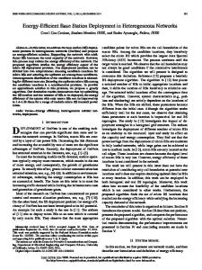
We use an example to illustrate how the algorithm CreatingClusters(V, k) works. Consider a wireless sensor network with 11 sensor nodes and 3 base stations as shown in Figure 1. Figure 1(a) shows the Voronoi diagram our algorithm creates. All the neighbouring nodes of I are E, D, H, and K, and all the neighbouring nodes of H are C, D, G, I, J and K. At the beginning, there are 6 clusters with each sensor being one cluster. Next, the algorithm merges a smallest cluster with its best neighbouring cluster at a time. Figure 1(b) shows the intermediate clusters created by the algorithm

Voronoi Cells F

4+5

5

3

J

F

J F

4

G A

1+5

J G

C

K

1

A

G

C

K

H

A

C

K

H

D

H

D

B

B

Clusters

2

I

D B

I

I 2+6

6

Sensor Node

E

E

(a)

(b)

E

(c)

Fig. 1: An example for illustrating the algorithm CreatingClusters(V, k).

CreatingClusters(V, k), where each cluster except the cluster I is merged from two clusters. For example, the cluster {C, F } is merged from the cluster {C} and the cluster {F }. Figure 1(c) shows the final clusters {A, B, C, F }, {D, E, I} and {G, J, H, K} created by our algorithm. In the second phase, the algorithm ClusterBalancing(C, L) aims to modify the initial clusters so that the maximum total shortest hop distance of any cluster is minimised, where C is the set of k initial clusters and L is the set of the optimal locations of the k base stations. It starts with the initial k clusters created by the algorithm CreatingClusters(V, k). In each iteration, a modifiable cluster Ci with the highest TSHD among all the clusters in C is selected. A cluster Ci is modifiable if there exist a neighbouring cluster Cs with TSHD(Cs )