Efficient Estimation of 3D Euclidean Distance Fields from ... - CiteSeerX

Efficient Estimation of 3D Euclidean Distance Fields from 2D Range Images Sarah F. Frisken and Ronald N. Perry Mitsubishi Electric Research Laboratories

ABSTRACT Several existing algorithms for reconstructing 3D models from range data first approximate the object’s 3D distance field to provide an implicit representation of the scanned object and then construct a surface model of the object using this distance field. In these existing approaches, computing and storing 3D distance values from range data contribute significantly to the computational and storage requirements. This paper presents an efficient method for estimating the 3D Euclidean distance field from 2D range images that can be used by any of these algorithms. The proposed method uses Adaptively Sampled Distance Fields to minimize the number of distance evaluations and significantly reduce storage requirements of the sampled distance field. The method is fast because much of the computation required to convert the line-of-sight range distances to Euclidean distances can be done during a pre-processing step in the 2D coordinate space of each range image. Keywords: distance fields, ADFs, 3D scanning, range images

1. INTRODUCTION There are many approaches for reconstructing 3D models from range data. Some comprehensive reviews of these approaches can be found in [Curless 1999, Whitaker 1998, and Edelsbrunner 2002]. Here we focus on methods that first compute an implicit representation of the surface, usually in the form of a sampled distance field, and then reconstruct the 3D model as an iso-surface of the implicit representation. While some of these methods are designed to be very general, e.g., they can accept range data in the form of an unorganized cloud of surface points, we focus on range data that is available in the form of range images, where range measurements are acquired in a regularly sampled 2D grid. Since many commercial scanners acquire data in this format, this focus is not overly limiting and allows us to exploit the available coherency between range values from the same range image. In this paper, we present an efficient method for computing 3D distance fields from 2D range images. The method approximates the Euclidean distance from line-of-sight distances of each range image and then combines distances from one or more scans to provide a final estimate of the true Euclidean distance. Justification for using Euclidean distances is based on reconstruction accuracy and speed and is presented in Section 3.2. Our method performs most of the computation in the 2D coordinate space of each range image during a preprocessing step, resulting in significant computational savings. In addition, the method represents the sampled distance field using octree-based Adaptively Sampled Distance Fields (ADFs) to minimize the number of distance evaluations and significantly reduce memory requirements.

2. BACKGROUND 2.1 Distance Fields An object’s distance field represents, for any point in space, the distance from that point to the object. The distance can be signed to distinguish between the inside and outside of an object. The metric used to measure distance can take many forms, but Euclidean distance is frequently used because of its utility in a number of applications (e.g., collision detection and surface offsetting). Distance fields are a specific example of implicit functions, which have a long history of use and study (e.g., see [Bloomenthal 1997]). Distance fields have been used in CAD/CAM [Ricci 1973, Rockwood 1989, Breen 1990, Schroeder et al. 1994, Perry and Frisken 2001], medical imaging and surgical simulation [Blum 1973, Raya and Udupa 1990, Payne and Toga 1990, Jones and Chen 1995, Szeliski and Lavalle 1996, Frisken-Gibson 1999], modeling deformation and animating deformable models [Bloomenthal and Wyville 1990, Bloomenthal and Shoemake 1991, Payne and Toga 1992, Gascuel 1993, Whitaker 1995, Sethian 1996, Cani-Gascuel 1998, DesBrun and Cani-Gascuel 1998, Breen 1998, Fisher and Lin 2001], scan conversion or ‘voxelization’ [Payne and Toga 1992, Jones 1996, Gibson 1998, Sramek and Kaufman 1999], robotics [e.g., Koditschek 1989], and have recently been advocated as a surface representation in their own right [Gibson 1998, Frisken et al. 2000]. Early work represented the distance field implicitly and operations on the distance field were computed from the implicit representation at query points as needed. More recent work uses volumetric methods, computing and storing distance values in a regular 3D grid and reconstructing distance values at non-grid locations using an interpolation method such as trilinear interpolation. Like all sampled representations, adequate sampling is required for alias free reconstruction of the sampled distance field, resulting in large memory requirements and slow processing times for detailed models. Several approaches have been made to reduce processing times and/or memory requirements. Recently [Hoff 1999, Hoff 2001] introduced hardware methods for fast computation of regularly sampled distance fields. Others reduce processing by restricting evaluation of the distance field to a ‘shell’ or ‘narrow band’ around the object surface [Curless 1996, Jones 1996, Desbrun 1998, and Whitaker 1998]. In some cases, accurate distance values evaluated in the shell are then propagated to voxels outside the shell using fast distance transforms [Jones 2001, Zhao et al. 2001] or fast marching methods from level sets [Kimmel and Sethian 1996, Breen et al. 1998, Whitaker 1998, and Fisher 2001]. [Szeliski and Lavalle 1996, Wheeler 1998, and Strain 1999] evaluate distance values at cell vertices of a classic or ‘3-color’ octree (i.e., an octree where all cells containing the surface are subdivided to the maximum octree level) to reduce the number of distance evaluations (over regular sampling) and to provide an estimate of the distance field away from the surface.

2.2 Adaptively Sampled Distance Fields More recently, it was observed that substantial savings both in memory requirements and in the number of distance evaluations

proach results in a substantial reduction in the number of distance evaluations and significantly fewer stored distance values than would be required by a 3-color quadtree. ADFs are a practical representation of distance fields that provide high quality surfaces, efficient processing, and a reasonable memory footprint. [Perry and Frisken 2001] demonstrates the practical utility of ADFs in a 3D sculpting system that provides real time volume editing and interactive ray casting on a desktop PC (Pentium IV processor) for volumetric models that have a resolution equivalent to a 2048x2048x2048 volume.

2.3 Reconstructing 3D Models from Range Data Using Distance Fields

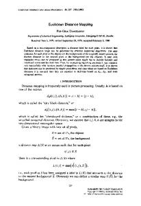
Figure 1. A 3-color quadtree of this 2D character requires 20,813 quadtree cells (top) while a quadtree-based ADF using a bi-quadratic interpolant of the same accuracy requires only 399 cells (bottom). Both quadtrees have a maximum level of 9, with resolution equivalent to a 512x512 image of distance values. 3D octree-based ADFs have similar compression in the 3rd dimension.

required to represent an object could be made by adaptively sampling the object’s distance field according to the local complexity of the distance field rather than whether or not a surface of the object was present. [Gibson 1998] noted that the distance field near planar surfaces can be reconstructed exactly from a small number of sample points using trilinear interpolation. This observation led to ADFs [Frisken et al. 2000], which use detail-directed sampling, i.e., high sampling rates where there are high frequencies in the distance field and low sampling rates where the distance field varies smoothly. As illustrated in Figure 1, this ap-

There are several methods for reconstructing 3D models from range data that make use of distance fields. Some of these methods make the general assumption that data is available only as an unorganized set of surface points. [Hoppe et al. 1992] creates a regularly sampled signed distance volume by defining local tangential planes from neighborhoods of scanned surface points and computing signed distances to these planes. Marching Cubes [Lorensen and Cline 1987] is then used to generate a surface model from the volume representation. [Edelsbrunner 2002, Bajaj et al. 1995, and Boissonnat and Cazals 2000] build Voronoi diagrams from scanned surface points. They then use the Voronoi diagram to efficiently evaluate closest distances to the surface and to define (initial) surface patches for the model. [Carr et al. 2001] fits a radial basis function to a set of on-surface and off-surface points derived from scanned surface points. The on-surface points are assigned a value of 0 while off-surface points constructed from the on-surface points are assigned a value equal to their signed distance from the surface. All of these methods are more general than the approach we discuss here because they can be applied to a set of unorganized points. However, when range data is available in the form of range images, these methods could make use of the efficient evaluation of the distance field that is described in this paper. [Curless and Levoy 1996, Hilton et al. 1996, and Wheeler et al. 1998] present methods that compute a volumetric representation of the distance field from range surfaces, which are created by connecting nearest neighbors in the range image with triangular facets. Triangulation over possible occlusions in the model surface is avoided by not connecting neighbors with significant differences in range values. This approach is conservative and avoids building surfaces over unobserved regions but can lead to holes in the model that must be addressed separately [Curless and Levoy 1996]. These three methods all use a weighted averaging scheme to combine distance values from multiple scans. As in [Hoppe et al. 1992], these methods use Marching Cubes to generate a triangle model from the volume representation. [Curless and Levoy 1996] uses line-of-sight distances and only compute distances in a limited shell surrounding the surface. The distance volume is run-length-encoded to reduce storage and processing times. [Hilton et al. 1996] computes Euclidean distances from range surfaces in a shell surrounding the surface, and stores the results in a regularly sampled volume. [Wheeler et al. 1998] also computes Euclidean distances from range surfaces but limits distance evaluations to the vertices of a 3-color octree. [Whitaker 1998] computes line-of-sight distances directly from range images and combines distance values from multiple scans using a windowed, weighted average. He then uses level set methods to reduce scanner noise by evolving a surface subject to forces that 1) attract it to the zero-valued iso-surface of the distance field and 2) satisfy a shape prior such as surface smoothness. [Zhao et al. 2001] uses a similar method to [Whitaker 1998], but initializes the

Range Image

Range Image dp-

Projected Distance, dp

dp+ Occluded Surface

True Distance, dt

Surface Profile

Surface Profile

Figure 2. Projected distances, dp, differ from the true Euclidean distance, dt, to a surface when the surface is at an angle to the scanning direction (left) and when there are occluded regions (right) where projected distances do not measure the distance to the occluded surface. Occluded regions result in discontinuities in the projected distance field (e.g., the discontinuity between the measurements dp- and dp+).

distance field used to attract the evolving surface from a set of unorganized points. Recently [Perry and Frisken 2001] and [Sagawa et al. 2001] describe a method similar to [Wheeler et al. 1998] but use ADFs instead of a 3-color octree to reduce the number of distance evaluations required. [Perry and Frisken 2001] uses an error predicate to guide adaptive subdivision of the ADF while [Sagawa et al. 2001] uses a measure of local surface curvature. Both papers introduce new methods for hole-free triangulation of the (un-restricted) octrees. [Sagawa et al. 2001] remeshes the octree to form a non-rectilinear grid that is free of T-junctions and uses an extension of Marching Cubes to generate the triangle model while [Perry and Frisken 2001] extend a method for triangulating regularly sampled binary data presented in [Gibson 1998].

Figure 3. Even for surfaces with relatively low curvature, the direction and magnitude of the gradient computed using central differences (red arrows) is significantly different from the true gradient (white arrows) (left). After correcting the distance field with the gradient magnitude, the computed gradient better approximates the true gradient of the distance field (right).

3. ESTIMATING EUCLIDEAN DISTANCE FROM 2D RANGE IMAGES 3.1 Projected Distances 2D range images provide a 2D grid of line-of-sight distances from the scanner to the object. In this paper, we assume that each value in the range image represents the perpendicular projected distance from the plane of the scanner to the object. Scanning systems do not always provide perpendicular projected distances but conversion to this form is often straightforward. As an example, laser striping systems fan a laser beam into a plane of laser light so that each range image scan line samples line-of-sight distances along rays radiating from the point laser source to the object. Given the geometry of the laser striping system and the angle of each ray to the laser source, these line-of-sight distances can be converted to perpendicular distances and mapped back onto the plane of the scanner. Resampling these mapped projected distances into a regular grid provides the required perpendicular projected range image. This conversion can result in some loss of data near occluded regions but the effect is usually small.

3.2 Why Euclidean Distances? While some prior work uses line-of-sight distances [e.g., Curless and Levoy 1996] or projected distances [e.g., Whitaker 1998], we advocate the use of Euclidean distances because 1) they provide a more accurate representation of both the direction to the surface for off-surface points and the surface itself when combining multiple scans, 2) they permit faster generation of the ADF (and hence the model), and 3) they provide better compression of the distance field in the ADF thus enabling the representation of high resolution models. The projected distance can vary significantly from the true Euclidean distance in two ways as illustrated in Figure 2. First, when the surface is at an angle to the scanning direction, the true distance value is smaller than the projected distance value. Second, the range image does not represent distances to occluded surfaces and surfaces that are nearly parallel with the scanning

Figure 4. Combining projected distances to a sphere from two scans (separated by 90 degrees) results in artifacts where the two scans overlap (left). After correcting the distance field with the gradient magnitude, these artifacts are significantly reduced (right).

direction. At such surfaces, projected distances in the range image are discontinuous and result in an interface in the projected distance field where large positive and large negative distances can be located in adjacent samples. While the projected distance field has the same zero-value iso-surface as the Euclidean distance field, the gradient of the projected distance field differs from the gradient of the true Euclidean distance field (see Figure 3, left). This can be problematic for methods that use the distance field gradient to evolve a surface towards the zero-value iso-surface. In addition, when multiple range images are combined, projected distances from different view directions are scaled differently. If the distances from all scans are linearly averaged, the resultant zero-valued iso-surface of the combined projected distances still represents the object surface accurately. However, most methods use a windowed, weighted, non-linear averaging of distance values from different scans. This results in artifacts in the surface where two scans overlap (see Figure 4, left). In addition to accuracy, there are practical reasons for preferring the Euclidean distance field when using ADFs. First, if we are primarily interested in the distance field near the surface, we can terminate cell subdivision early during ADF generation when a cell is guaranteed not to contain the surface. With Euclidean distances, where distance values are proportional to cell size, it is easy to determine if a cell cannot contain the surface from the cell’s distance values (e.g., if every cell distance value has the same sign AND the absolute magnitude of every cell distance value is greater than one half the cell diagonal, then the cell is

Scanning Direction

Scanning Direction dp z

θ

N

dt θ

N

x y

Plane Equation: Ax + By + Cz + D = 0 Normal: N = (A, B, C)

dt = dp cos(θ)

Figure 5. The true distance to a planar surface (left) is equal to the projected distance multiplied by cos(θ), where θ is the angle between the scanning direction and the surface normal. For a planar surface (right), it is shown in the text that the magnitude of the gradient of the projected distance field is equal to 1/cos(θ).

either interior or exterior). However, projected distances are not proportional to cell size: they are scaled depending on the angle of the surface to the scanner’s line-of-sight and are discontinuous near occluded surfaces. Hence, using projected distances precludes the use of terminating cell subdivision early and typically requires more than an order of magnitude more distance evaluations and significant temporary storage during ADF generation. A second reason for preferring Euclidean distances is that with a projected distance field, discontinuities near occluded surfaces force cells near these occluded surfaces to be subdivided to the highest level of the ADF, resulting in memory requirements similar to that of a 3-color octree.

3.3 Correcting Projected Distances As illustrated on the left in Figure 5, for points near a planar surface, the Euclidean distance, dt, is equal to the projected distance, dp, multiplied by cos(θ) where θ is the angle between the scanning direction and the surface normal, i.e., dt = dp ∗ cos(θ). Given the plane on the right in Figure 5, the projected distance, dp, from a point p = (p.x, p.y, p.z) to the plane along the z direction is dp = p.z – (– p.x ∗ A/C – p.y ∗ B/C – D/C). Differentiating, the gradient of the projected distance field, ∇(dp), is ∇(dp) = (A/C, B/C, 1), with magnitude, |∇(dp)| = (A2 + B2 + C2)1/2 / C. Because the plane’s normal is (A, B, C), cos(θ) is equal to C/(A2 + B2 + C2)1/2. Hence, |∇(dp)| = 1 / cos(θ) and, for planar surfaces, dt = dp ∗ cos(θ) = dp / |∇(dp)|, i.e., we can correct the projected distance field near relatively planar regions of the surface by dividing the projected distance by the magnitude of the local gradient of the projected distance field. This correction results in a better approximation of the Euclidean distance near smooth surfaces. Making this correction for a regularly sampled volume is straightforward (but slow): we sample the projected distance field for each point in the 3D volume to create a projected distance volume and then correct the projected distance at each sample point by dividing by the local gradient magnitude computed using, for example, central differences. However, for ADFs, computing the local gradient of the projected distance field during generation is inefficient since it requires evaluating 6 additional distances per ADF sample point that might not otherwise be required. To avoid these unnecessary distance evaluations, we observe that in the direction perpendicular to the range image, the projected distance to the object decreases at a constant rate. Hence,

the gradient of the projected distance field is constant along rays perpendicular to the range image. This means that the gradient of the 3D projected distance field can be fully represented by a 2D field in the plane of the range image. Figure 6 provides pseudocode for evaluating this 2D field to produce a 2D gradient magnitude correction image. The gradient magnitude correction image is pre-computed prior to ADF generation at the same resolution as the range image. During generation, a projected distance value is derived from the range image and corrected using a value interpolated from its corresponding pre-computed gradient magnitude correction image as described in Section 3.5. CreateGradientMagnitudeCorrectionImage(rangeImage[NxM]) { //----Compute the inverse gradient magnitude correction image float invGradMagCorrection[NxM] xScale Å 0.5 * rangeImageWidth yScale Å 0.5 * rangeImageHeight for (pixel = each range image pixel) { dx Å xScale * (rangeImage[x+1] – rangeImage[x-1]) dy Å yScale * (rangeImage[y+1] – rangeImage[y-1]) gradMag Å sqrt(dx^2 + dy^2 + 1.0) invGradMagCorrection[pixel] Å 1 / gradMag } }

Figure 6. Pseudocode for the gradient magnitude correction image.

3.4 Correcting Distances Near Cliffs Range values are discontinuous between pixels in the range image near occluded surfaces (Figure 2, right) and near surfaces that run approximately parallel to the scanning direction. Existing approaches that use range surfaces handle these discontinuities by not triangulating over these pixels. However, this results in holes in the range surface and possibly in the resultant 3D model that must be treated specially by the algorithm or addressed separately. Here, instead of discarding data near these discontinuities, we make the assumption that the surface is continuous across a range image discontinuity, and forms a “cliff” that runs perpendicular to the range image connecting pixels on each side of the discontinuity. This approach eliminates holes in the reconstructed surface and provides a reasonable guess at regions of the surface for which there is no data available. Note that this method does not necessarily provide accurate distances to occluded surfaces. Therefore, we assign a low priority to distances computed from cliffs when combining multiple scans (Section 3.5) so that distances from range images with better views of an occluded region are favored over cliff distances. To correct the distance field near cliffs during ADF generation, we locate the nearest cliff for each ADF sample point and choose the smaller of the gradient magnitude corrected distance and the distance to the cliff. Cliff pixels – pixels that are beside a discontinuity in the range image – can be detected and marked in a pre-processing step. However, computing cliff distances may seem like an ominous task – recall that we propose using cliff distances to remove discontinuities in the 3D distance field in order to reduce generation times. Even if we bin cliff pixels in a spatial hierarchy and use a fast search technique to locate nearest cliff pixels it is hard to imagine that this approach would provide much improvement over simply requiring complete 3-color octree subdivision of the ADF along the cliffs. Fortunately, similar to gradient magnitude correction, 3D cliff distances can be estimated from an (annotated) 2D image that can be computed prior to generation. This annotated 2D image, or “cliffmap”, encodes distances to the top and bottom of the nearest cliff for each pixel in the range image as well as the heights of the top and bottom of that cliff. During generation we interpolate the 2D cliffmap to estimate cliff distances for each 3D sample point in the ADF. We

use the top and bottom heights of the nearest cliff to determine the Euclidean distance to the cliff. Figure 7 provides pseudocode for computing the 2D cliffmap from a range image. CreateCliffCorrectionImages(rangeImage[NxM]) { float cliffTopHeight[NxM] // Range value of closest top and float cliffBotHeight[NxM] // bottom cliff pixels. float cliffTopDist[NxM] // Horizontal distance to closest top float cliffBotDist[NxM] // and bottom cliff pixels. //----Compute the cliff images. First detect the top and bottom //----cliff pixels, set their heights and set their cliff //----distances to zero. for (pixel = each range image pixel) { //----Initialize pixel as a non-cliff pixel cliffTopDist[pixel], cliffBotDist[pixel] Å ∞ //----Check the 8 neighbors of this pixel to see if there is a //----change in intensity greater than cliffThreshold. If so, //----this is a cliff pixel. for (neighbor = each of pixel’s 8 neighbors) { dif Å rangeImage[pixel] – rangeImage[neighbor] if (dif > cliffThreshold) { //----This is a top cliff pixel cliffTopHeight[pixel] Å rangeImage[pixel] cliffTopDist[pixel] Å 0 } else if (dif < -cliffThreshold) { //----This is a bottom cliff pixel cliffBotHeight[pixel] Å rangeImage[pixel] cliffBotDist[pixel] Å 0 } } } //----Reduce contiguous 1-pixel wide cliffs to a single multi//----pixel wide cliff by setting pixels tagged as both top and //----bottom cliffs to non-cliff pixels for (pixel = each cliff pixel) { if (!cliffTopDist[pixel] && !cliffBotDist[pixel]) { cliffTopDist[pixel], cliffBotDist[pixel] Å ∞ } }

single range image are 1) compute the projected distance at p from the range image, 2) compute the associated gradient magnitude from the pre-computed gradient magnitude correction image and correct the projected distance value, 3) compute the distance to the nearest cliff using the pre-computed cliffmap, and 4) choose the smaller of the corrected projected distance and the cliff distance. Steps 2) – 4) are detailed in the pseudocode of Figure 8. Distances from multiple scans can be combined in several ways depending on the method used for reconstructing surfaces. For example, one could use any of the weighted averaging schemes proposed by [Curless and Levoy 1996, Hilton et al. 1996, Wheeler et al. 1998, and Whitaker 1998]. The best combining method is determined by the noise characteristics of the range scanner and any further processing applied by the reconstruction method. For purposes of illustration, we use a simple combining scheme that chooses the ‘best’ distance value from multiple scans where ‘best’ means that small distance values are favored over large distance values, distance values with small gradient magnitudes are favored over distance values with large gradient magnitudes, and corrected projected distances are favored over cliff distances. This method was used to reconstruct the model of Figure 12 (see Section 3.7). GetCorrectedDist(projDist, p) { //----Compute the gradient magnitude corrected distance value invGradMag Å GetInterpolatedValue(invGradMagArray, p) dist Å projDist * invGradMag //----Interpolate heights and distances to the nearest cliff //----from the cliffmap topDist Å GetInterpolatedValue(cliffTopDist, p) botDist Å GetInterpolatedValue(cliffBotDist, p) top Å GetInterpolatedValue(cliffTopHeight, p) bot Å GetInterpolatedValue(cliffBotHeight, p)

//----Initialize unsigned distances from cliff pixels using a //----distance transform such as a 3x3 neighborhood Euclidean //----transform, e.g., apply the following to each pixel in the //----cliffmap twice, processing first left to right, bottom //----to top and then right to left, top to bottom. for (pixel = each cliffmap pixel) { for (neighbor = each of pixel’s 8 neighbors) { dist Å cliffTopDist[pixel] nbrDist Å cliffTopDist[neighbor] + EuclidDistToNbr cliffTopDist[pixel] Å min(dist, nbrDist) dist Å cliffBotDist[pixel] nbrDist Å cliffBotDist[neighbor] + EuclidDistToNbr cliffBotDist[pixel] Å min(dist, nbrDist) } }

//----Determine the distance to the nearby cliff and compare it //----to the gradient magnitude corrected distance. Keep the //----smaller distance. The distance to the cliff depends on //----whether the sample point is above the top of the cliff, //----below the bottom of the cliff, or in-between. z Å p.z if ((dzToTop = top - z) dist) dist Å d } else if ((dzToBot = z - bot)