Efficient estimation of two-dimensional firing rate surfaces via ...

Efficient, adaptive estimation of two-dimensional firing rate surfaces via Gaussian process methods Kamiar Rahnama Rad and Liam Paninski Department of Statistics and Center for Theoretical Neuroscience Columbia University June 18, 2010 Abstract Estimating two-dimensional firing rate maps is a common problem, arising in a number of contexts: the estimation of place fields in hippocampus, the analysis of temporally nonstationary tuning curves in sensory and motor areas, the estimation of firing rates following spike-triggered covariance analyses, etc. Here we introduce methods based on Gaussian process nonparametric Bayesian techniques for estimating these two-dimensional rate maps. These techniques offer a number of advantages: the estimates may be computed efficiently, come equipped with natural errorbars, adapt their smoothness automatically to the local density and informativeness of the observed data, and permit direct fitting of the model hyperparameters (e.g., the prior smoothness of the rate map) via maximum marginal likelihood. We illustrate the flexibility and performance of the new techniques on a variety of simulated and real data.

1

Introduction

A common problem in statistical neural data analysis is to estimate the firing rate of a neuron given some two-dimensional variable. Spatial examples include the estimation of “place fields” in the hippocampus (Brown et al., 1998), “grid fields” in entorhinal cortex (Hafting et al., 2005), and position- or velocity-fields in motor cortex (Gao et al., 2002; Paninski et al., 2004a). Spatiotemporal examples include the estimation of tuning curves that change as a function of time (Frank et al., 2002; Rokni et al., 2007); purely temporal examples include models of spike-history effects (Kass and Ventura, 2001) or the tracking of firing rates that change as a function of both intra- and inter-trial times during a behavioral task (Czanner et al., 2008). Finally, more abstract examples arise in the context of spike-triggered covariance analyses (Rust et al., 2005; Aguera y Arcas and Fairhall, 2003). More generally, the estimation of the intensity function of two-dimensional point processes is a central problem in a variety of other scientific fields, including forestry and astronomy (Moeller and Waagepetersen, 2004). A number of methods have appeared in the literature to address this problem. It is worth briefly reviewing some of these approaches here, in order to illustrate some of the computational and statistical aspects of this two-dimensional point-process smoothing problem. Perhaps the most direct (and common) approach is to write p(spike|~x), the conditional probability of observing a spike in a small time bin given the two-dimensional signal ~x, as p(spike|~x) = 1

p(spike, ~x) , p(~x)

and then to estimate the probability densities in the numerator and denominator via standard nonparametric methods, either via histogram or kernel smoothing methods (Devroye and Lugosi, 2001); thus our estimate of the conditional firing rate is obtained as a ratio of estimated densities pˆ(spike, ~x)/ˆ p(~x). The advantages of this method include its conceptual simplicity and its computational speed; in particular, linear smoothing methods for obtaining pˆ(spike, ~x) and pˆ(~x) essentially involve a standard spatial convolution operation, which may be computed efficiently via the fast Fourier transform. Also, uncertainty in the estimated firing rates can be quantified via standard bootstrap methods (though this may be computationally expensive). However, the disadvantages of this approach are quite well-known (Kass et al., 2003; Kass et al., 2005): if the kernel width (or histogram bin) in the density estimate is chosen to be too large, then the estimated firing rate surface is oversmoothed; on the other hand, if the kernel width is too small, then the division by the small, noisy estimated density pˆ(~x) can lead to large, noisy fluctuations which can mask the underlying structure in the estimated firing rate. Another important but somewhat more subtle disadvantage of this direct ratio approach has to do with the “adaptivity” of the estimator. Speaking roughly, we would like our estimator to smooth out the data more in areas where fewer observations are available (and where the estimate is bound to be noisier), while letting the data “speak for itself” and applying minimal smoothing in regions where many ~x observations are available (where reliable estimates can be made without too much spatial averaging). The ratio estimator as described above does not have this important adaptive property. It is of course possible to make this smoother adaptive: one method is to let the kernel width scale roughly inversely with the number of samples ~x observed in a local region. However, this method is somewhat ad hoc; more importantly, since this adaptive smoothing can not be computed via a simple convolution, the fast Fourier methods no longer apply, making the method much slower and therefore obviating one of the main advantages of this ratio approach. Finally, it is well-known that the firing rate typically depends not just on a single location variable ~x, but also on additional covariates, e.g., the time since the last spike (Berry and Meister, 1998; Kass and Ventura, 2001; Frank et al., 2002; Paninski, 2004), or the local activity of other cells in the network (Harris et al., 2003; Paninski et al., 2004b; Truccolo et al., 2005; Paninski et al., 2007; Pillow et al., 2008); it is difficult to systematically incorporate these covariate effects in the simple nonparametric ratio approach. Parametric statistical models lie at the other end of the spectrum. We may model the firing rate p(spike|~x) ≈ p(spike|~x, θ), where θ is a finite-dimensional parameter, and then fit θ directly to the observed data via standard likelihood-based methods (Brown et al., 1998; Kass et al., 2005). Confidence intervals on the estimated firing rates may again be obtained by bootstrapping, or by the standard likelihood asymptotic methods based on the observed Fisher information (though this approach is only effective when many data observations are available and, more importantly, when the model is known to provide a good explanation of the data); in addition, it is easy to incorporate covariates (e.g., the effect of the local spike history). Parametric methods can be very powerful when a good model is available, but the results are highly dependent on the model family chosen. For example, two-dimensional unimodal Gaussian surface models for place fields can be effective for some hippocampal cells, but fail badly when modeling grid cells, which display many bumps in their firing rate surfaces. Computation in parametric models involves optimization over the parameter θ, and therefore typically scales like O(dim(θ)3 ); this adverse scaling encourages researchers to

2

reduce the dimensionality of θ, at the expense of model flexibility1 . Finally, local maxima in the model’s objective function surface can be a significant concern in some cases. State-space methods for estimating time-varying tuning curves represent something of a compromise between these two approaches (Brown et al., 2001; Frank et al., 2002; Czanner et al., 2008; Paninski et al., 2009). These methods are quite effective in the spatiotemporal cases cited above, but do not apply directly to the purely spatial setting. The idea is to fit a parametric model to the tuning curve, but then to track the changes in this tuning curve as a function of time using what amounts to a temporal smoothing method. These methods can be cast in a fully Bayesian setting that permits the calculation of various measures of uncertainty of the estimated firing rates and the incorporation of our prior knowledge about the smoothness of the firing rate in time and space. Computation in these methods scales roughly as O(dim(θ)3 T ) (Paninski et al., 2009), where θ again represents the model parameter and T represents the number of time points at which we are estimating the firing rate. In this paper we discuss a Bayesian nonparametric approach to the two-dimensional pointprocess smoothing problem which is applicable in both the spatial and spatiotemporal settings. Our methods are in a sense a generalization of the temporal state-space methods for point process smoothing; we will see that very similar local computational properties can be exploited in the spatial case. The resulting estimator is adaptive in the sense described above, comes equipped with confidence intervals, and can be computed efficiently. Our methods may also be considered a generalization of the techniques described by (Gao et al., 2002), and as a computationally efficient relative of the techniques considered in (Cunningham et al., 2007; Cunningham et al., 2008). We will discuss the relationship to this work below in more depth, after describing our methods in more detail.

2

Methods

2.1

The doubly stochastic point process model

We model neural activity as a point process with rate λ, with λ depending smoothly on some two-dimensional variable ~x. For technical reasons which we will discuss further below, we will model the firing rate in terms of a smooth nonnegative function f (.) applied to a two-dimensional surface z(~x); this surface z(~x), in turn, is assumed to be a smooth function which we will estimate from the observed point process data. Thus, the firing rate map λ(~x) = f (z(~x)) will itself be a smooth nonnegative function of ~x. We will study several somewhat distinct experimental settings and show that they all can be conveniently cast in these basic terms. The experimental settings we have in mind are: 1. We observe a spatial point process whose rate is given by λ(~x) = f [z(~x)]. 2. We observe a temporal point process whose rate is given by λt = f [z(~xt )], where ~xt is some known time-varying path through space (e.g., the time-varying position of a rat in a maze (Brown et al., 1998) or the hand position in a motor experiment (Paninski et al., 2004b)). 1

The typical O(dim(θ)3 ) complexity is due to the matrix-solve step involved in Newton-Raphson optimization over the parameter θ. Solving a linear equation involving a N ×N matrix leads to the O(N 3 ) computational complexity.

3

3. We make repeated observations of a temporal point process whose mean rate function (i) may change somewhat from trial to trial2 ; in this case we may model the rate as λt , where t denotes the time within a trial and i denotes the trial number (Frank et al., 2002; Czanner et al., 2008). 4. We observe a temporal process whose rate is given by λ(t) = f [z(x(t), t)], where x(t) is some known time-varying path through a one-dimensional space (e.g., the time-varying position of a rat in a linear maze), and the one-dimensional tuning curve f [z(x, t)] changes as a function of time (Frank et al., 2002; Rokni et al., 2007). 5. We observe a temporal process whose rate is given by λ(t) = f [z(t, τ )], where z(t, τ ) depends on absolute time t and the time since the last spike τ . Models of this general form are discussed in (Kass and Ventura, 2001), who termed these “inhomogeneous Markov interval” models. We provide detailed formulations for each of the mentioned applications in appendix A. Each of these formulations may be elaborated by the inclusion of additional terms, as we discuss in section 2.6 below. In all cases, the nonnegative function f (.) is assumed to be convex and log-concave (Paninski, 2004). We further model z as a sample from a Gaussian process with covariance function C(~x, ~x′ ) (Cressie, 1993; Rasmussen and Williams, 2006); as we discuss below, this allows us to encode our a priori assumptions about the smoothness of z in a convenient, flexible fashion3 . In this setting, the resulting point process is doubly-stochastic and is known as a Cox process (Snyder and Miller, 1991; Moeller and Waagepetersen, 2004); in the special case that f (.) = exp(.), the process is called a log-Gaussian Cox process (Moeller et al., 1998). Related models have seen several applications in the fields of neural information processing and neural data analysis (Smith and Brown, 2003; Jackson, 2004; Brockwell et al., 2004; Sahani, 1999; Wu et al., 2004; Wu et al., 2006; Yu et al., 2006); for example, the temporal point-process smoothing methods developed by Brown and colleagues (Frank et al., 2002; Smith and Brown, 2003; Czanner et al., 2008) may be interpreted in this framework. In particular, as mentioned above, (Gao et al., 2002) and (Cunningham et al., 2007; Cunningham et al., 2008) applied similar techniques to the problem of estimating spatial receptive fields; we will discuss the relationship to this work in more depth in the discussion section below.

2.2

Smoothing priors

To set the stage for our main development over the next two sections, it is helpful to review some concepts in Bayesian smoothing and estimation. There is a very large statistical literature on smoothing in one and more dimensions (Wahba, 1990; Green and Silverman, 1994). For conceptual simplicity, let’s begin by reviewing the one-dimensional smoothing problem from a Bayesian point of view. In this setting we have a univariate sequential ordered series y1 , y2 , · · · , yn observed at locations τ1 , τ2 , · · · , τn on a one-dimensional grid. The goal is to approximate this series by a smooth continuous function z(τ ), i.e. yi = z(τi ) + ǫi , 2

(1)

Thanks to C. Shalizi for pointing out this example. We will discuss the advantages of placing the prior on z, instead of directly on the firing rate f (z), in the next sections. 3

4

where ǫi is measurement error. Assuming that equation (1) is the true model and the measurement error is Gaussian with zero mean and variance σ 2 , the probability of the observed data D = {yi }i=1,··· ,n given the smooth continuous function z(τ ) is given by: p(D|z) = (2πσ 2 )−n/2

n Y

e−

(yi −z(τi ))2 2σ 2

.

(2)

i=1

The maximum likelihood estimate zM L (τi ) = yi is obtained by maximizing the logarithm of equation (2) over z(τi ) for i = 1, · · · , n. Unfortunately, the resulting estimate is not necessarily a smooth continuous function; in fact, in this case the MLE is not even well-defined except at the observed points τ = τi , since the likelihood does not depend on z(τ ) for τ 6= τi . The standard approach for remedying this problem is to introduce a functional of z(.) to penalize non-smooth functions: zˆγ = arg max log P (D|z) − γF(z). z

(3)

The first term accounts for the fit of the data, while the second penalizes the roughness of z(τ ). The functional F(z) must be bigger forR non-smooth functions z(.) compared to smooth ∂z 2 functions. One common choice for F(.) is [ ∂τ ] dτ , the total power of the first derivative (Wahba, 1990). Another common choice for F(.) is the integrated length of the square of the second derivative which gives greater smoothness than the first derivative constraint. The tuning parameter γ > 0 exists to balance fitness (in terms of log-likelihood) versus smoothness (in terms of integrated square of the first derivative). In the limit of small γ the estimate zˆγ (.) better fits the data and is less smooth. As we increase the tuning parameter, zˆγ (.) becomes smoother but fits the data less well. The tuning parameter may be chosen by hand (using our a priori knowledge of the smoothness of the function z), or by any of several existing databased methods, such as generalized cross validation, expectation maximization, generalized maximum likelihood or empirical Bayes (Wahba, 1990; Hastie et al., 2001). From a Bayesian point of view, the penalizing term can be interpreted as a prior on z(.): log P (z|γ) ∝ −γF(z). Since P (z|D, γ) ∝ P (D|z)P (z|γ) as a function z(.), the maximum a posteriori (MAP) estimate of z(.) is given by zˆγ

= arg max P (z|D, γ) z

= arg max log P (D|z) + log P (z|γ), z

which is equivalent to (3) when log P (z|γ) ∝ −γF(z). Likewise, priors based on smoothing constraints can be used to estimate two-dimensional surfaces given point process observations. The motivation is as in the one-dimensional Gaussian case: without any prior on smoothness, estimating the rate map (by maximizing the loglikelihood) results in a jagged, discontinuous rate surface with singularities on the observed spikes. One simple and convenient prior penalizes large differences in the two-dimensional surface z, exactly as we discussed above in the one-dimensional case:  Z  ∂ 2 ∂ 2 ( z) + ( z) dxdy, log P (z(.)|γ) ∝ −γF(z) = −γ (4) ∂x ∂y 5

4

5 50

1

10

2

15

100

3

2 1

20

0

3

150 25

1 200

2

3

−1

30 50

100

150

200

10

20

30

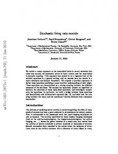
Figure 1: Example of the inverse prior covariance matrix C −1 , with γ = 1 and ǫ = 0. The penalty functional F(z) is implemented via a quadratic form z T C −1 z; choosing the inverse prior covariance C −1 to be sparse banded allows us to efficiently compute the posterior ˆ Left: The banded structure of C −1 , in an example setting where z is expected firing rate λ. represented as a 10 × 20 grid. Middle: The first 30 × 30 entries of C −1 . Right: The five-point “stencil” implemented in C −1 ; note that only nearest spatial neighbors are involved in the computation of the penalty.

where ~x = (x, y) and z = z(~x). If F(z) is close to zero, then z will be smooth (Wahba, 1990). Three brief technical points are worth noting here. First, this R prior is not a proper probability distribution because it can not be normalized to one (i.e., exp[−γF(z)]dz = ∞.). However, in most cases the posterior distribution P (z(.)|D, γ) will still be integrable even if we use such an improper prior (Gelman et al., 2003). Note that to take into account the a priori boundedness of z(~x) we may augment the roughness penalty in a simple way:  Z  Z ∂ 2 ∂ 2 ˜ ( z) + ( z) dxdy + ǫ z 2 dxdy; F(z) = (5) ∂x ∂y ˜ this small extra term makes P (z|γ) ∝ exp[−γ F(z)] a proper prior. The scalar ǫ here sets the inverse scale of z: smaller values of ǫ correspond to larger prior variance in the Gaussian prior specified by log P (z|γ). Second, it is possible to tune the smoothness along the horizontal and vertical directions independently. This is useful when the two dimensions are measured in different units (e.g., time and location). This is easily done by introducing two roughness tuning parameters as follows:  Z  ∂ 2 ∂ 2 γx ( z) + γy ( z) dxdy. F(z) = (6) ∂x ∂y Third, it is possible to consider penalties based on higher derivatives, as in the one dimensional case (Wahba, 1990). For example, the penalty of equation (6) based on the second derivative is as follows:  Z  ∂2z 2 ∂2z 2 γx ( 2 ) + γy ( 2 ) dxdy. F2 (z) = ∂x ∂y As before, the MAP estimate of z is defined as:

˜ zˆγ = arg max{log P (D|z) + γ F(z)}. z

6

−4 0

50 100

−4.5 −3.5

−0.5

150 200

−3

−5 −4

−1 100

200

−5.5 100

200

−4.5 100

200

Figure 2: Three independent samples z drawn from the Gaussian prior with covariance matrix C and mean zero, with γ = 20 and ǫ = 10− 6. Note that samples can take a fairly arbitrary shape, though slowly-varying (correlated) structure is visible in each case.

(We will introduce the likelihood P (D|z) for the point process case in the next section.) To implement this estimator numerically, we must discretize space and represent the function z in vector form. We may simply discretize the spatial variable ~x and then concatenate the resulting matrix z by appending its columns to construct a vector4 . In the discrete domain, any of the aforementioned penalties can be written in terms of quadratic forms in the vector z, i.e. as z T C −1 z for an appropriate sparse positive semi-definite matrix C −1 . See Figure 1 for an example of C −1 such that z T C −1 z implements F(z) for a surface z which is represented in the discrete domain on a 10 × 20 grid. Note that the exact form of C in the case where the prior log P (z|γ) ∝ −z T C −1 z is improper may not exist. This is due to the fact that some of the eigenvalues of C −1 may be zero in which case C does not exist. It is important to remember that the Gaussian prior corresponding to the exponent of the negative quadratic penalty z T C −1 z only acts as a regularizer, and does not imply that we are modeling the random surface z(~x) as a single Gaussian-shaped bump as a function of the two-dimensional spatial variable ~x; instead, p(z) is a Gaussian function of the much higher-dimensional vector z, and therefore in general samples z from this prior may have quite arbitrary multimodal shapes as a function of ~x, as illustrated in Fig. 2.

2.3

Computing the posterior

Now our main goal is to efficiently perform computations with the posterior distribution p(z|D) of the random surface z given the observed spike train data D5 . For example, given p(z|D) we can estimate the firing rate by taking the conditional expectation Z
ˆ x) = E f [z(~x)]|D = f (u)p(z(~x) = u|D)du. λ(~ It is well-known that for convex and log-concave f (.) the log-posterior log p(z|D) = log p(D|z) + log p(z) + const. 4

With a slight abuse of notation we interchangeably use z for both the vector representation and the grid representation. The difference should be clear from the context. 5 Note that the posterior depends on the prior which itself is function of the hyper-parameter γ discussed in the previous section. All the posterior probabilities for the rest of the paper are for a fixed γ unless otherwise mentioned and to simplify notation we discard the dependence on γ.

7

is concave as a function of z (Paninski, 2004; Paninski, 2005; Cunningham et al., 2007), since both the prior p(z) and the point-process likelihood p(D|z) are log-concave in z 6 , and logconcavity is preserved under multiplication. As a result log p(z|D) has no non-global local maxima in z, and therefore standard gradient ascent algorithms are guaranteed to converge to a global maximum if one exists. Furthermore, this log-concavity allows the development of efficient approximation and sampling algorithms for the posterior p(z|D) using the Laplace approximation (Ahmadian et al., 2009; Kass and Raftery, 1995), as we discuss below. As mentioned earlier, we assume a Gaussian prior on z: log p(z) = −z T C −1 z + const.

(7)

The inverse covariance matrix C −1 encodes both the smoothness and boundedness of z, as discussed in the previous section. Now our basic approximation is a standard Laplace approximation (Fahrmeir and Kaufmann, 1991; Kass and Raftery, 1995; Paninski et al., 2007) for the posterior:   1 1 T −1 p(z|D) ≈ (8) exp − (z − zˆD ) CD (z − zˆD ) , 2 (2π)d/2 |CD |1/2 where d = dim(z), zˆD = arg max p(z|D) z

and −1 CD = C −1 + HD ,

(9)

with HD = −∇∇z log p(D|z)z=ˆzD . In words, this is just a second-order approximation of the concave function log p(z|D) about its peak zˆD . We have found that this approximation is acceptably accurate when the log-prior and log-likelihood are smooth and concave, as is the case here; see e.g. (Paninski et al., 2009; Pillow et al., 2009; Ahmadian et al., 2009) for further discussion. Two items are worth noting. First, zˆD may be found via ascending the objective function log p(z|D) by the Newton-Raphson algorithm. Since this function is concave and is therefore unimodal, as emphasized above, we don’t need to worry about local maxima. In principle finding the maximum of a concave function is straightforward (Boyd and Vandenberghe, 2004). The difficulty arises when the dimensionality of z is large which in our applications −1 might be as large as ∼ 105 . Second, CD is quite easy to compute once we have zˆD , since HD is a diagonal matrix (as can be demonstrated by explicit computation; see equation (11) below). The key to computing the posterior distribution in equation (8) is to develop efficient methods for computing zˆD . The standard Newton-Raphson ascent method requires that we solve the linear equation
(10) C −1 − ∇∇z log p(D|z)z=ˆz (i) w = ∇z log p(z|D)z=ˆz (i) 6

The point-process log-likelihood is given generically as (Snyder and Miller, 1991) Z T X log p(D|z) = log λ(ti ) − λ(t)dt, 0

i

where ti are the observed spike times and [0, T ] is the time interval over which the spike train is observed; for details on how to compute the likelihood in each of the settings mentioned in section 2.1, see Appendix A.

8

for the search direction w, where zˆ(i) denotes our estimate of z after i iterations of NewtonRaphson. For example, in the simplest setting (case 1 described in section 2.1), we have the standard point-process log-likelihood (Snyder and Miller, 1991) Z X log p(D|z) = log f [z(~xj )] − f [z(~x)]d~x + const. j

where j indexes the location ~xj where the j-th spike was observed, and so X f′ ∂ log p(D|z) = −f ′ [z(~x)]d~x + [z(~x)]δ(~x − ~xj ) ∂z(~x) f j

and ∂ 2 log p(D|z) = ∂z(~x)∂z(~x′ )

(

−f ′′ [z(~x)]d~x + 0

P

j

f ′′ f −(f ′ )2 [z(~x)]δ(~x f2

− ~xj )

if ~x = ~x′ otherwise,

(11)

where f ′ (.) and f ′′ (.) denote the first and second (scalar) derivatives of the function f (.). Note that if f (.) = exp(.), the second term of the first line in equation (11) is zero. So the feasibility of this smoothing method rests primarily on the tractability of the Newton step (10), which in turn rests on our ability to solve equations of the form
C −1 + H w = b

as a function of the unknown vector w, for diagonal matrices H. For general d × d matrices C −1 , this will require O(d3 ) time7 , which is intractable for reasonably-sized z. (Cunningham et al., 2007; Cunningham et al., 2008) introduced techniques for speeding up the computations in this general case to find an approximate MAP estimate of the rate map which behaved reasonably well in numerical examples; we take a different approach here and restrict our attention to a special subclass of covariance functions C which is flexible enough for our needs but at the same time allows us to perform the necessary computations much more efficiently than in the general O(d3 ) case. Before we discuss these computational issues, though, it is worth mentioning a few imporˆ for the firing rate. First, the Bayesian approach tant statistical properties of the estimator λ ˆ (as allows to systematically calculate various measures of the uncertainty of the estimator λ we will discuss at more length below), and it is straightforward to incorporate our prior knowledge about the smoothness of z in the definition of the covariance function C. In addition, the Bayesian estimator, by construction, functions as an adaptive smoother: because the Bayesian estimator represents a balance between the data and our prior beliefs about z, the estimator will smooth less in regions where the data are highly informative, and vice versa. Quantitatively, this balance of data versus prior is determined by the size of the “observed Fisher information matrix” HD compared to the inverse prior covariance C −1 , and therefore depends both on the observed data and the nonlinear function f (.); for f (.) = exp(.), for example, HD increases with the firing rate, since λ(u) = f ′′ (u) is monotonically increasing in u, and therefore the effective smoothing width decreases in regions of high firing rate, as desired. More concretely, when the observed information matrix HD is large compared to 7 Note that computing HD requires just O(T ) time, where T is the length of the experiment, and therefore this step is not rate-limiting.

9

the prior covariance C, the posterior uncertainty (measured by the posterior covariance CD , −1 equation (9)) is approximately HD , whereas the posterior uncertainty reverts to the prior uncertainty (i.e., C) when the observed data D are less informative. This adaptive behavior can also be understood by examining the matrix equation (10) in the Fourier domain: since the inverse covariance C −1 is typically chosen to penalize high-frequency fluctuations (Theunissen et al., 2001), larger values of the diagonal term HD correspond to a local spatial filter (C −1 + HD )−1 which passes higher spatial frequencies, and which is therefore more spatially localized (Paninski, 2005).

2.4

Priors based on nearest-neighbor penalties lead to fast computation

In this section we will describe how to choose the inverse prior covariance C −1 so that we can solve the Newton step in a computationally efficient manner while retaining the statistical efficiency and biological plausibility8 of our estimator. The basic insight here is that if [C −1 ]~x,~y = 0 whenever ~x and ~y are not neighbors on the discrete two-dimensional grid9 , then C −1 may be written in block-tridiagonal form with tridiagonal blocks, and our equation resembles a discrete Poisson equation, for which highly efficient multigrid solvers are available which require just O(d) time (Press et al., 1992). Even standard methods for solving the equation (as implemented, e.g., in Matlab’s A\b call) are quite efficient here, requiring just O(d3/2 ) time10 . We have found that a very simple Newton-Raphson algorithm exploiting these efficient linear algebra techniques (and a simple backtracking method to ensure that the objective increases with each Newton step) converges in just a few iterations, therefore providing a rapid and stable algorithm for computing zˆD ; the optimization takes just a few seconds on a laptop computer for d ∼ 104 . In contrast, if we represent z in some finitedimensional basis set B in which fast matrix solving methods are not available, then each Newton step generically requires O(dim(B)3 ) time. Thus we see that the fast sparse matrix techniques allow us to investigate spatial receptive fields of much higher resolution, since d may be made much larger than dim(B) at the same computational cost. Once zˆD is obtained using these efficient methods, we estimate the firing rate map by: Z Z E[f (z(~x))|D] = f (u)p(z(~x) = u|D)du ≈ GzˆD (~x),Var[z(~x)|D] (u)f (u)du, where we have applied the Laplace approximation in the second step and abbreviated the Gaussian density in u with mean µ and variance σ 2 as Gµ,σ2 (u). In the case that f (.) = exp(.), f [z(~x)] has a lognormal distribution and we may read off the conditional mean E[f (z(~x))|D] and variance Var[f (z(~x))|D] using standard results about this distribution; for example,   1 (12) E[exp(z(~x))|D] = exp zˆD (~x) + Var[z(~x)|D] . 2 8

Biological plausibility refers here to the exclusion of sharp discontinuities and singularities in the rate map. In examples considered in this paper we will focus mainly on the nearest-neighbor case, but the methods may be applied more generally when [C −1 ]~x,~y = 0 if ~x and ~ y are separated by a distance of more than n pixels, where n is small (n = 1 in the nearest-neighbor case). 10 This O(d3/2 ) scaling requires that a good ordering is found to minimize fill-in during the forward sweep of the Gaussian elimination algorithm; code to find such a good ordering (via “approximate minimum degree” algorithms (Davis, 2006)) is built into the Matlab call A\b when A is represented as a sparse banded matrix. See also (Sanches et al., 2008) for an approach based on a related Sylvester equation; this approach is quite different but turns out to have the same computational complexity. 9

10

In any case, we need to compute the conditional variances Var[z(~x)|D], which under the Laplace approximation are given by the diagonal elements of CD . These terms may be computed without ever computing the full matrix CD (which would require O(d2 ) storage) −1 by making use of the banded structure of CD , via standard algorithms such as the forwardbackward Kalman smoother or the method described in (Asif and Moura, 2005). This step requires O(d2 ) time. However, in many cases (as we will see below), Var[z(~x)|D] is somewhat smoother than E[z(~x)|D], and may therefore be computed on a coarser scale (making d smaller) and then interpolated to a finer scale; thus this O(d2 ) time scaling is not a major limitation. Another important R application of the Laplace approximation is to compute the marginal likelihood p(D|θ) = p(z, D|θ)dz, where θ denotes parameters we might want to optimize over in the context of model selection (e.g., the hyperparameters setting the spatial scale and variance of the prior covariance C; see Results section below), or in constructing hierarchical models of the observed rate maps over multiple neurons (Behseta et al., 2005; Geffen et al., 2009). The Laplace approximation for this marginal likelihood is Z 1 −1 log p(D|θ) = log p(D, z|θ)dz ≈ log p(ˆ zD |θ) + log p(D|ˆ zD , θ) − log |CD | + const., (13) 2 where “const.” is constant in θ and the dependence of zˆD (and therefore HD ) on θ has been left implicit to avoid cluttering the notation. The first two terms here are easy to compute once zˆD has been obtained: the first (Gaussian) term is a sparse banded quadratic form, and the second is the usual point-process loglikelihood. The third term requires the determinant of a sparse banded matrix, which again may be computed efficiently and stably via a Cholesky decomposition; the “chol” function in Matlab again automatically takes advantage of the −1 sparse banded nature of CD here, and requires just O(d3/2 ) time. It is also worth noting that the generalization to non-Gaussian priors of the form   X p(z) ∝ exp  hij [z(~xi ) − z(~xj )] , ij

for some collection of smooth, symmetric, concave functions hij (.), is straightforward, since the log-posterior remains smooth and concave. For example, by using sub-quadratic penalty functions hij (.) we can capture sharper edge effects than in the Gaussian prior (Gao et al., 2002); conversely, if we use penalty functions of the form ( 0 |u| < K , hij (u) = −∞ otherwise then we may directly impose Lipschitz constraints on z (Coleman and Sarma, 2007) (the resulting concave objective function is non-smooth, but may be optimized stably via interiorpoint methods (Boyd and Vandenberghe, 2004; Cunningham et al., 2007; Cunningham et al., 2008; Vogelstein et al., 2008; Koyama and Paninski, 2009; Paninski et al., 2009)). Once again, to maintain the sparse banded structure of the Hessian C −1 + H we choose hij (.) to be uniformly zero for non-neighboring (~xi , ~xj ). We recover the Gaussian case if we choose hij (.) to be quadratic with negative curvature; in this case, the nonzero elements of the inverse prior covariance matrix (C −1 )ij correspond to the pairs (i, j) for which the functions hij (.) are not uniformly zero. 11

2.5

MCMC methods

While we have found the Laplace approximation to be quite effective in the applications we have studied (Ahmadian et al., 2009), in many cases it may be useful to draw samples from the posterior distribution p(z|D) directly, either for Monte Carlo computation of the ˆ or for visualization and model checking purposes. The prewhitened firing rate estimator λ Metropolis-adjusted Langevin or hybrid Monte Carlo algorithms (Robert and Casella, 2005; Ahmadian et al., 2009) are standard MCMC algorithms that are well-suited for sampling from the near-Gaussian posterior p(z|D). To implement this algorithm here, we only need an efficient method for solving the prewhitening equation Rw = η for w, where η is a standard normal sample vector and R is the Cholesky decomposition of −1 CD . As noted above, R may be computed in O(d3/2 ) time here, and each call to the solver for Rw = η again requires just O(d3/2 ) time, although due to the high dimensionality of z here the chain may require many steps to mix properly (Robert and Casella, 2005; Ahmadian et al., 2009). We have not explored this approach extensively.

2.6

Using the Schur complement to handle non-banded cases

There are two important settings where our sparse banded matrix methods need to be modified slightly. First, in some cases we would like to impose periodic boundary conditions on ˆ For example, (Rokni et al., 2007) analyzed the dynamics of tuning curves as our estimate λ. ˆ should also a function of arm direction; since direction is a periodic variable, our estimate λ be periodic in the direction, for all values of time (i.e., we have to impose “cylindrical” — ˆ We can ensure periodperiodic in direction but not in time — boundary conditions on λ). ˆ icity in our estimate λ simply by choosing our inverse prior covariance matrix C −1 to have −1 the desired cylindrical boundary conditions. However, this means that CD no longer has a banded form; the upper-right and lower-left corner blocks of this matrix are nonzero. Our second example involves the inclusion of covariate information. Each of the experimental settings introduced in section 2.1 may be elaborated by including additional covariate information (e.g., spike history effects (Paninski, 2004; Truccolo et al., 2005)). For example, instead of modeling the rate of our observed temporal point process as λ(t) = f [z(~x)], we could use the model λ(t) = f [z(~x) + Wt θ] instead, where W denotes a matrix of known (fixed) covariates and θ is a set of weights we would like to fit simultaneously with z. We can proceed by directly optimizing log p(z, θ|D) (assuming θ has a log-concave prior which is independent of z); this joint optimization in (θ, z) is tractable, again, due to the special structure of the Hessian matrix of the objective function log p(z, θ|D) here. the parameter vector  If we order T Hzz Hθz , where Hzz has the as {z, θ}, the Hessian may be written in block form H = Hθz Hθθ special sparse banded form discussed above. Thus,  in both ofthese examples we have to solve a linear equation involving a block matrix H11 H12 H = , where the size of the block H11 is much larger than that of the block T H12 H22 H22 , and the large block H11 is sparse banded. These systems may be solved easily in O(d3/2 ) time via Schur complement methods; for details see appendix B and for an illustration see Figure 9 below. 12

True Rate

Path

Est. Rate

y

−1 −0.8

−0.8

−0.6

−0.6

−0.4

−0.4

−0.2

−0.2

0

0

0.2

0.2

0.4

0.4

0.6

0.6

0.8

0.8

25

20

15

10

1

−1

5

−0.5

0

0.5

1

Kernel Estimator, σ=0.1

Std. Rate

Kernel Estimator, σ=0.05

−1 −0.8 −0.6 −0.4

y

−0.2 0 0.2 0.4 0.6 0.8 1 −1

−0.5

0 x

0.5

1

−1

−0.5

0 x

0.5

1

−1

−0.5

0 x

Figure 3: Estimating the two-dimensional firing rate given a spike train observed simultaneously with a time-varying path ~x(t). The simulation was done with 10ms time bins and a total of ∼ 2800 spikes over 600 seconds. Top left: The true firing rate surface λ(~x). Top middle: The trace of the path ~x(t) through the two dimensional space for the first 10 seconds with red dots indicating the spikes. Top right: The posterior expectation of the firing rate surface, i.e. E [f (z)|D]. Bottom left: The posterior standard deviation of the firing rate surface. Bottom middle and right: The kernel estimator with isotropic bandwidth σ = 0.1 and σ = 0.05, respectively. For small bandwidth the kernel estimator is very noisy, especially at the corners, where no samples are available.

3

Results

In this section we will describe several applications of the methods described above, to both simulated and real spike train data. In all examples we find the posterior expectation of the firing rate map by equation (12). We assume that f (.) = exp(.) and use log p(z) ∝ −γF(z), as defined in equation (4). Recall that any convex and log-concave f (.), e.g. log(1 + ex ), could be used instead of the exponential non-linearity. All hyper-parameters γ are estimated by the empirical Bayes method described in appendix D.

13

0.5

1

Posterior std. of z

MAP estimate of z

True z

−1 3

−0.8 −0.6

2.5 −0.4 2

−0.2 0

1.5 0.2 1

0.4 0.6

0.5 0.8 1 −1

0 −0.5

0

0.5

1

−1

−0.5

0

0.5

1

−1

−0.5

0

0.5

Figure 4: The spatial fields z(x, y) corresponding to the estimated firing rates λ(x, y) shown in Fig. 3; units are dimensionless and correspond to variations in the log-firing rate. Note that in this figure the posterior standard deviation and the MAP estimate of the latent surface z is presented as opposed to figure 3 which presents the posterior expectations of firing rate surface, i.e. E [f (z)|D]. Left: The posterior standard deviation of z(x, y), i.e. std [z|D], which is smaller around the center because more samples are available from that region (c.f. the top middle panel of Figure (3)). Middle: The MAP estimate of z(x, y). Right: The true z(x, y).

3.1 3.1.1

Synthetic data A two-dimensional spatial place field

We begin with the second example introduced in section 2.1: we observe a temporal point process whose rate is given by λ(t) = exp[z(~x(t))], where ~x(t) is a (known) time-varying path through space. ~x(t) was sampled from two dimensional random walk. The unknown underlying random two-dimensional surface z(~x) is assumed to be constant in time. The experiment we are trying to simulate is the estimation of the firing rate surface of a single grid cell from the recorded spike train of the corresponding cell. Figure 4 illustrates an estimated place field: we see that the method provides a very accurate estimate of the true z(x, y) for centrally-located points ~x, where the space has been sampled densely (see the top middle panel of Figure 3). For more peripheral points ~x, on the other hand, less data are available. Here the estimated firing rate relies more heavily on the prior, and reverts to a flat surface (since a gradient-penalizing prior, as discussed in section 2.2, was used here). As emphasized above, these estimates are computationally efficient, requiring just a few seconds on a laptop computer to recover surfaces zˆ described by ∼ 104 parameters. The middle bottom and right bottom panel of Figure 3 shows the results of the popular Gaussian kernel estimator (see appendix C for details). As we increase the bandwidth of the Gaussian kernel the estimate becomes smoother. The kernel estimator performs poorly in this example mainly because it is not able to adapt its bandwidth according to the local informativeness of the observations and only a sparse sample is available. The performance of the kernel estimator is much better in the case that observations of all points in the domain of interest are available, as we will see in section 3.1.3.

14

1

3.1.2

A temporally-varying one-dimensional spatial field

Next we examine setting 4 from section 2.1. Here we have a one dimensional tuning curve which changes with time. In this example z is placed on a 100 × 200 grid. The experiment we are trying to simulate is the estimation of temporally varying tuning curve from a single cell recording. This can correspond to the estimation of the one dimensional spatial receptive field of cell which changes over time while the rat is running back and forth on a one dimensional track. We observe a sample path, xt (which was sampled from a one dimensional random walk), along with a point process of rate λ(t) = f [z(xt , t)]; the resulting estimate of the underlying spatiotemporal firing rate is shown in Figure 5. Similar results as in Figure 3 are obtained: as long as the path samples the space enough, we obtain a reasonable estimate of the changing tuning curve but where insufficient data are available the estimator reverts to the prior. As before, we assume that f (.) = exp(.) and R ∂z
2 R ∂z
2 dxdt − γt dxdt. The hyper-parameters γx and γt were estiuse log p(z) ∝ −γx ∂x ∂t mated using the empirical Bayes method explained in appendix D. Figure 6 shows the result of the linear Gaussian kernel smoothing with different combinations of temporal and spatial bandwidths. The kernel estimator is more problematic in this application; the output of this estimator depends heavily on the sample path xt . Of course the Bayesian estimate also depends on the path, but this estimator is better able to balance the information gained from the data with our prior information about the smoothness of the rate map. 3.1.3

Trial-by-trial firing rate modulations

Finally, we analyze the simulated example data involving the between-trial and within-trial neural spiking dynamics (as in setting 3 in section 2.1) from (Czanner et al., 2008); this data set was simulated to emulate recorded data from a monkey performing a location-scene association task. See the top left panel of Figure 7 for the simulated spike train over 50 trials: this model neuron displays strong non-stationarity both within and between trials. For N trials each having duration T δ, we use the following model: P (D|z) =

T N Y Y e−f (zi,t +Hi,t )δ (f (zi,t + Hi,t )δ)ni,t

ni,t !

i=1 t=1

,

where ni,t stands for the number of spikes within the the interval (tδ, (t + 1)δ] in the ith trial, δ for bin size, and T the number of bins in one trial. The history effect is defined by: Hi,t =

τ X

ht′ ni,t−t′ ,

t′ =1

where ht stands for the spike history term and τ for its duration; τ = 30 ms here, following (Czanner et al., 2008). Note that z(i, t) lies on a N × T grid which is a 104 dimensional space because of N = 50 and T = 200. The estimate of (z, h) is found by the joint optimization ) ( −1 h X NX 2 i  2 γt  ˆ = arg max log P (D|z, h) + , z(i, t + δ) − z(i, t) (ˆ z , h) γn z(i + 1, t) − z(i, t) + z,h δ t n=1 (14) where the hyper-parameters γn and γt determine how strongly the estimate is smoothed across trials and within trials, respectively. The hyper-parameters are estimated using the 15

True rate

Posterior expectation of the rate

−1

Rat location

−0.5

120

120

100

100

80

80

60

60

40

40

20

20

0

0.5

1

Posterior standard deviation 30 140 25

Spikes/bin

120 20

100

15

80 60

10

40 5 20 0

0

20

40

60

80

100

120

140

160

180

200

20

Bins(100ms)

40

60

80

100

120

140

160

180

200

Time(100ms)

Figure 5: Estimating a one-dimensional time varying spatial tuning curve. Top left: The actual color map of the rate surface as a function of location and time (color) and the observed one-dimensional path of the animal as a function of time (black trace). Top right: The posterior expectation of the rate for a 20s period with a total of ∼ 1300 spikes. The rate map as a function of location and time is observed very sparsely and for areas like the top right or the bottom middle of the rate map no observations are available as is clear from the path of the animal. The posterior expectation of the rate map at unobserved parts is effectively smoothed based on observations from other parts. Note in particular that in the upper right, where no data are available, the estimate reverts to the prior, which forces the inferred rate to be a flat extrapolation of the observed data from the right middle of the rate map. Bottom left: Observed spike count. Bottom right: The posterior standard deviation of the firing rate surface. The standard deviation increases with the firing rate (c.f. Eq. 12) and is higher at the lower half and top right part where limited data are available; c.f. the black path shown in the top left panel.

empirical Bayes method described in appendix D. The joint optimization is performed using the methods discussed in section 2.6; once zˆ is found it is straightforward to calculate the posterior expectation and standard deviation of the rate map as described in section 2.4. See Figure 7 for data, results and comparisons. The latent surface z and the history term ht were estimated simultaneously. However, for the estimated firing rate maps shown in the middle panel of figure 7 the effect of the spiking history, which varies much more sharply as 16

σ =0.2sec and σ=0.1

σ =0.5sec and σ=0.2

t

t

−1

Rat location

−0.5

120

120

100

100

80

80

60

60

40

40

20

20

0

0.5

1

σ =0.5sec and σ=0.1

σ =0.2sec and σ=0.2

t

t

−1

Rat location

−0.5

120

120

100

100

80

80

60

60

40

40

20

20

0

0.5

1 20

40

60

80

100

120

140

160

180

200

20

Time(100ms)

40

60

80

100

120

140

160

180

200

Times(100ms)

Figure 6: Kernel estimator of the one-dimensional time varying spatial tuning curve of Figure 5. Each panel corresponds to a different combination of spatial and temporal bandwidth. For small bandwidths (e.g., top left panel), the estimate is quite noisy. The dark blue blocks seen in the top and bottom left figures are due to the fact that we don’t have enough samples from those regions and that the bandwidth is small (i.e., the estimate is undefined at these locations). As we increase the bandwidth this problem seems to disappear but still the map is heavily influenced by the path of the animal; c.f. the black path shown in in the top left panel of Figure 5.

a function of time t than does the latent surface z, is excluded from this plot, to emphasize what was specifically referred to as the “stimulus component” (in our terminology, the zdependent component) of the firing rate surface in (Czanner et al., 2008). The posterior expected rate map (middle left panel of Figure 7) and the simple kernel estimator (bottom right panel of Figure 7) provide qualitatively similar results, since in this case we have an observation for every point on the rate grid (unlike the case analyzed in Figs. 5-6). The smooth posterior expectation here illustrates the power of sharing statistical information both within and between trials. The state-space method implemented in (Czanner et al., 2008) (middle right panel of Figure 7), on the other hand, only smooths across trials, not across neighboring time bins, and therefore leads to a much noisier estimate11 . 11

More concretely, the state-space method discussed in (Czanner et al., 2008) may be understood as a version of the Gaussian process method discussed here (Paninski et al., 2009): the state-space term encodes a Gaussian prior on a latent variable which modulates the firing rate in an exponential manner, exactly as in our model if we take f (.) = exp(.). The major difference is that (Czanner et al., 2008) choose their statespace model parameters such that the the corresponding prior inverse covariance matrix C −1 lacks the second

17

The marginal loglikelihood log P (D|γn , γt ) of the hyper-parameters (γn , γt ) is shown in the top right panel of Figure 7. In appendix D we describe how to efficiently estimate this marginal likelihood. By plotting the marginal log likelihood of the hyper-parameters over a grid it is possible to choose the best values of these smoothing hyper-parameters, as is shown in the top right panel of Figure 7. The influence of the hyper-parameters on zˆ is clear from Figure 8; as we increase γn (top rows to bottom rows), smoothing across trials becomes stronger. Likewise the right columns are smoother over time compared to the left ones.

3.2

Real data

3.2.1

Two dimensional spatial firing map

Now we apply our methods to data previously analyzed in (Paninski et al., 2004a; Paninski et al., 2004b). In these experiments, a monkey was trained to manually track a moving target on a two-dimensional plane, guided by visual feedback on a computer monitor. The hand position ~x(t) was recorded simultaneously with the spike trains of several neurons in the primary motor cortex (MI). As is well-known, MI neurons are tuned to a variety of kinematic variables, including the hand position, velocity, and acceleration. To explore the nonlinear properties of MI tuning to these variables, we fit a model of the form λ(t) = f [Wt θ + z(~x(t))], where the six-column covariate matrix   ∂~x(t) ∂ 2 ~x(t) Wt = ~x(t) ∂t ∂t2 contains the observed time-varying horizontal and vertical position, velocity, and acceleration, and θ denotes a six-dimensional set of linear weights acting on Wt . By including the linear terms Wt θ in the model and by using the gradient penalty in the prior for z, we ensure that the estimated z(~x) contains only nonlinear effects as a function of ~x, since any linear trend will be accounted for by the Wt θ term. More precisely, any linear trend in z has non-zero gradient and will therefore be penalized, whereas this linear dependence is parametrically included in Wt θ, which is unpenalized here. Therefore, the estimate of z will not show any linear dependence, allowing us to isolate any non-linear dependence in z. Note that z lies on a 100 × 100 grid. The results are shown in Figure 9; we see that, as reported in (Paninski et al., 2004b), the tuning here is largely linear in Wt and the non-linear dependence which is captured by z is less significant compared to the linear dependence. (Similar results were observed in other cells and when z was allowed to depend on velocity instead of position; data not shown.)

4

Discussion

We have introduced Gaussian process methods for estimating the conditional intensity function of two-dimensional point processes, and demonstrated the application of these methods in a variety of neural coding settings. Our basic approach was to approximate the posterior term in the r.h.s. of equation (14), which enforces smoothness across neighboring time bins. (Specifically, in their implementation the state-space covariance matrix Σ = cov(ǫk ) is diagonal, so the firing rate is estimated independently in each time bin; see (Czanner et al., 2008) for notation and details.) There are also more minor differences in the computation of the posterior expectation of the firing rate; see (Paninski et al., 2009) for further discussion.

18

Figure 7: Estimating the firing rate in the context of significant trial-to-trial nonstationarity. Top left: The observed spike trains for different trials; see (Czanner et al., 2008) for simulation details. Top right: The log of the marginal likelihood of the hyper-parameters γt and γn ; the empirical Bayes method discussed in appendix D chooses the “best” smoothing parameters by maximizing this function. Middle left: Posterior expectation of the firing rate, i.e. E [f (z)|D] which in (Czanner et al., 2008) was specifically mentioned as the stimulus component of the firing rate, computed using hyper-parameters (γt , γn ) chosen via empirical Bayes (i.e., maximizing the surface shown in the top right panel). This estimated model (including the estimated history effects Hi,t , not shown here) passed the Kolmogorov-Smirnov goodness of fit test described in (Brown et al., 2002) at the 99% level. Middle right: Smoothed estimate using the method discussed in (Czanner et al., 2008). This estimate of the firing rate surface was referred to as the “stimulus component” in (Czanner et al., 2008). Again, for clarity, the latent variable z and the history term were estimated jointly but we only show the “stimulus component” (excluding the discontinuous spike-history effect) here. Bottom left: The posterior standard deviation of the estimated firing rate surface, using the same hyperparameters as in the middle left panel. Bottom right: output of kernel smoother. The time bandwidth and trial bandwidth are 100ms and 3 trials, respectively. Note that the kernel and Bayesian methods seem to perform well here; the state-space method of (Czanner et al., 2008) seems to undersmooth the data in the t direction.

19

γt=3.98

γt=63.1

γ=15.85

γt=251.19

γt=1000

γn=2.51

γn=0.63

γn=0.16

γn=0.04

γn=0.01

γt=1

γn=10

8 6 4 2 0

Figure 8: Estimating the latent surface z(t, n) in the context of significant trial-to-trial nonstationarity, for different settings of the hyper-parameters (γt , γn ), as in eq. (14). The top rows correspond to smaller γn and bottom ones to bigger γn ; the left columns correspond to smaller γt and right columns to bigger γt . To be concrete, γt increases logarithmically from 1 to 1000 from the left columns to the right columns. Similarly, γn increases logarithmically from 0.01 to 10 from the top rows to the bottom rows. As we increase γn the smoothing across trials becomes stronger. Similarly, by increasing γt the temporal smoothing becomes stronger. Figure 7, upper right, displays the corresponding marginal log-likelihood for each of these hyperparameter settings.

distribution of the rate map using the Laplace approximation constructed by finding the MAP estimate and the Hessian at that point. The prior was chosen to enforce local smoothness while retaining the computational efficiency of the Newton-Raphson ascent method used to find the MAP estimate. Our work is closest to that of (Gao et al., 2002), (Czanner et al., 2008), and (Cunningham et al., 2007; Cunningham et al., 2008). We presented an explicit comparison of our method with that of (Czanner et al., 2008) in section 3.1.3 above. (Gao et al., 2002) discussed the estimation of two-dimensional firing rates in the context of motor cortical data recorded in the same experiments as the data shown in Figure 9; this previous work emphasized the importance of nearest-neighbor smoothing penalties to obtain valid estimates of the firing 20

est. rate

raw data 5

25 10

20

4

10

3

y

15 15

10 5

20

15

2 1

20 10

std. rate

15

20

0

non−linear PF 8

10

−0.6 10

−0.8

6 y

−1 4

15

15

−1.2 −1.4

2 20

−1.6

20 10

15

20

10

x

15

20

x

Figure 9: Estimating the nonlinearity in the position-dependent firing rate of an MI neuron. The data and predictions are confined to the indicated circles. Top left: Predicted firing rate of a single neuron as a function of position at zero velocity and acceleration, estimated via the Bayesian methods discussed here. Top right: The number of spikes in 50ms windows at different points in the position space. (The striped appearance here is due to aliasing effects, and should be ignored.) Bottom left: The standard deviation of the predicted firing rate. Note that the posterior uncertainty increases towards the more sparsely-sampled perimeter. Bottom right: The nonlinear part (z(~x)) of the estimated place-field. Note the very small scale of the nonlinear effect compared to the linear trend shown in the top left panel, consistent with the results of (Paninski et al., 2004b).

rate, and also discussed the relative benefits of quadratic vs. sub-quadratic penalty functions for recovering sharper features in the estimated rate surfaces. We have extended this work here by casting these methods in a Gaussian process setting, which allows us to provide estimates of the posterior uncertainty and of the marginal likelihood of the observed data. This framework allowed us to approach a number of additional applications, going beyond the estimation of a single spatial rate map. Our work focused especially on the computational efficiency of these techniques: we emphasized the log-concavity of the posterior and the use

21

of efficient linear algebra methods for optimization. We also developed methods to include additional covariate information in the estimates, and discussed the use of non-quadratic penalizers (as introduced by (Gao et al., 2002)) within the same computationally-efficient paradigm. The work of (Cunningham et al., 2007; Cunningham et al., 2008) is even closer in spirit to ours12 ; the Bayesian viewpoint is emphasized throughout in that paper. The major difference is that (Cunningham et al., 2007; Cunningham et al., 2008) tackled the case of fairly general covariance functions, whereas we have limited our attention to covariance functions whose inverses contain only local potentials; this restriction allows us to exploit efficient computational linear algebra methods and makes our estimator significantly faster. (The beneficial computational properties of the banded matrices that result from these local potentials are of course well-known and exploited extensively in the spline literature (Wahba, 1990).) One additional technical difference is that (Cunningham et al., 2007; Cunningham et al., 2008) imposed nonnegativity constraints directly on the Gaussian process, instead of mapping the Gaussian process through a rectifying function f (.) as we have done here. This direct positivity-conditioning approach makes inference of the conditional mean and variance of the firing rate somewhat more difficult, since the marginal distribution of the multidimensional truncated Gaussian distribution is difficult to approximate (whereas in the case treated in this paper we can compute the mean and conditional variance of the estimated firing rate ˆ analytically, under the Laplace approximation). (Cunningham et al., 2007; Cunningham λ et al., 2008) used the MAP estimate to approximate the conditional expectation of the firing rate; this approximation is valid in the “high-information” limit, where the data likelihood dominates the variability of the prior. In cases where less data are available, MCMC techniques such as the hit-and-run algorithm (Lovasz and Vempala, 2003) can be employed to sample efficiently from the log-concave posterior distribution, though the “corners” due to the positivity prior enforced in (Cunningham et al., 2007; Cunningham et al., 2008) cause the MCMC chain to mix more slowly than in the case of the smooth posterior in the current work (Ahmadian et al., 2009). Recently, a fast nonparametric rate estimation method (Brown et al., 2009a; Brown et al., 2009b) based on variance stabilization transforms was introduced with desirable theoretical optimality properties. The variance stabilization transform turns the relatively complicated problem into a standard homoscedastic Gaussian regression problem and then any good nonparametric Gaussian regression procedure (e.g., wavelet smoothing) can be applied. One interesting direction for future work would be to combine the favorable properties enjoyed by this completely nonparametric method with those enjoyed by our Bayesian method; for example, it is not clear how to incorporate inhomogeneous observations (as described, for example, in Figs. 5-6 here) or additional covariate effects into the variance-stabilization method. We should also note that a number of fully-Bayesian methods have been developed to perform point-process smoothing in the one-dimensional case; the Bayesian adaptive regression splines (BARS) method described in (DiMatteo et al., 2001; Kass et al., 2003) is perhaps the most popular in the neuroscience community. These methods are based on MCMC integration over a suitable posterior and often provide state-of-the-art estimation accuracy, but at signif12

We should also mention (Cressie and Johannesson, 2008; Macke et al., 2010) here, who discuss yet another major alternative method for speeding computation in spatial Gaussian process models, in this case via imposing a low-rank structure on the prior covariance which may then be exploited computationally via the Woodbury matrix lemma. See (Cressie, 1993; Rasmussen and Williams, 2006) for further background and discussion.

22

icantly greater computational cost than the optimization approach pursued here. Extensions of the BARS method to the two-dimensional case are feasible but have not yet been pursued, to our knowledge; we would expect that the fast two-dimensional Laplace approximation methods we have developed here would be useful in this extended BARS setting. Finally, we should note that there are a number of well-known connections between the point-process and density estimation problems. Gaussian process methods for density estimation have been explored intensively in the statistics and physics literature (Good and Gaskins, 1971; Thorburn, 1986; Bialek et al., 1996; Holy, 1997; Schmidt, 2000; Paninski, 2005). One interesting avenue for future work would be to explore the application of the computational methods developed here to problems in two-dimensional density and conditional density estimation.

A

Detailed formulations of the different experimental setups

Here we discuss the experimental settings introduced in section 2.1 in somewhat more detail. 1. We observe a spatial point process on a grid whose rate is given by λ(~x) = f [z(~x)]. The likelihood of the observed spike train is given by: P (D|z) =

Y e−λ(~xi )δx (λ(~xi )δx)ni ni !

i

,

where the product is over all points of the grid and δx is the spatial binwidth and ni is the number of spikes observed in the i-th bin. 2. We observe a temporal point process whose rate is given by λt = f [z(~xt )], where ~xt is some known time-varying path through space (e.g., the time-varying position of a rat in a maze (Brown et al., 1998) or the hand position in a motor experiment (Paninski et al., 2004b)). Here the likelihood is given by P (D|z) =

T Y e−λt δt (λt δt)nt t=0

nt !

,

(15)

where the path of the animal during [0, T δt] does not necessarily cover all points of the grid. This setting is different from the first one in two ways. First, the time-varying path through space might not cover the whole space, and therefore we typically will not have observations for every point in space. Second, given the observed temporal spiking activity we are able to include the spiking history in the model (Paninski, 2004; Truccolo et al., 2005). In this case we have: λt = f [z(~xt ) + Ht ],

(16)

P where Ht = i ht−ti ; here ti is time of the ith spike and ht designates the spikehistory waveform. Note that we can generalize this model by adding other time-varying covariates, as discussed in section 2.6. 3. We make repeated observations of a temporal point process whose mean rate function (i) may change from trial to trial; in this case we may model the rate as λt , where t 23

denotes the time within a trial and i denotes the trial number. For N trials each having duration δtTi , we have: P (D|z) =

(i) Ti −λ(i) δt (i) N Y Y e t (λ δt)nt

i=1 t=0

t (i) nt !

,

(i)

where nt stands for the number of spikes within the (tδt , (t + 1)δt ] timebin of the ith trial. 4. We observe a temporal process whose rate is given by λ(t) = f [z(x(t), t)], where x(t) is some known time-varying path through a one-dimensional space. P (D|z) is given by equation (15). Here the two dimensions correspond to time and the one dimensional position, i.e. λ(x, t) = f (x, t). However, since the path x is changing over time we represented the firing rate as λ(t) = f (xt , t). 5. We observe a temporal process whose rate is given by λ(t) = f [z(t, τ )], where z(t, τ ) depends on absolute time t and the time since the last spike τ (Kass and Ventura, 2001). Imagine we observe the spike train {ti }i=1,··· ,l over a period of [0 δtT ] seconds. The likelihood is given by ! l R δtT Y P (D|z) ∝ e− 0 f [z(t,t−τ (t))]dt f [z(ti , ti − ti−1 )] f [z(t1 , ∞)] , i=2

where τ (t) is the time since last spike from time t and l the total number of spikes over a period of [0 δtT ]. In the discrete domain, for small enough δt such that the number of spikes nt in (tδt, (t + 1)δt] is either zero or one, we have: log P (D|z) ≈

B

T X l=0

nt log f [z(lδt, τ (lδt))] + (1 − nt ) log (1 − f [z(lδt, τ (lδt))δt]) + const.

Schur complement to handle non-banded matrices

As discussed in section 2.6, in some cases we have to solve the linear equation Hx = b,  H11 H12 , where the size of the block H11 is much larger involving a block matrix H = T H12 H22 than that of the block H22 , and the large block H11 is sparse banded. We have   −1 −1 T H −1 H )−1 H T H −1 −H −1 H (H − H T H −1 H )−1 H11 + H11 H12 (H22 − H12 12 12 22 12 −1 12 12 11 11 11 11 . H = T H −1 H )−1 T H −1 H )−1 H T H −1 (H22 − H12 −(H22 − H12 12 12 12 11 11 11 

Write x and b as (xT1 xT2 )T and (bT1 bT2 )T , respectively. We have −1 −1 −1 −1 −1 −1 T T T x1 = H11 b1 + H11 H12 (H22 − H12 H11 H12 )−1 H12 H11 b1 − H11 H12 (H22 − H12 H11 H12 )−1 b2 ,

−1 −1 −1 T T T x2 = −(H22 − H12 H11 H12 )−1 H12 H11 b1 + (H22 − H12 H11 H12 )−1 b2 .

24

Assume H11 is d × d and H12 is d × k, where d >> k or more specifically k = O(1). Finding −1 H11 y for any y takes O(d3/2 ), therefore by writing −1 −1 −1 T −1 T −1 −1 T (H22 − H12 H11 H12 )−1 = H22 − H22 H12 (H11 + H12 H22 H12 ) H12 H22 , T H −1 H )−1 y for any y in O(d3/2 ) and therefore x and x can be one can find (H22 − H12 12 1 2 11 −1 3/2 found in O(d ). Note that we want to avoid calculating H11 because of the storage cost.

C

Kernel Estimator

For every point ~x, let the empirical frequency of visits to that point and the relative frequency of observed spikes be designated by m~x and rP ~ x , respectively; thus the total number of observed spikes at ~x is m~x r~x . Further, let M stand for ~r′ m~r′ where the summation is over all points in the domain. Write p(n~x = 1|~x), for n~x ∈ {0, 1} as the indicator of a spike, as p(n~x = 1, ~x)/p(~x). One method to estimate p(~x) and p(n~x = 1|~x) is to build a histogram of the relative frequency of appearance of the empirical data. Instead the kernel estimator uses a smoothed estimate of the histogram as follows: X m~x′ k(~x, ~x′ ) pˆ(~x) = M ~ x′ X r~x m~x′ pˆ(n~x = 1|~x) = k(~x, ~x′ ), M ′ ~ x

where k(~x, ~x′ ) is called the kernel. For example the Gaussian kernel is defined as k(~x, ~x′ ) = √

1 2πσ 2

e−

k~ x−~ x ′ k2 2σ 2

,

and σ is the bandwidth parameter to control the smoothness of the estimate. The kernel estimator of the conditional probability simplifies to: P x, ~x′ ) x′ k(~ x′ m~ ~ x′ r~ pˆ(n~x = 1|~x) = P . x, ~x′ ) x′ k(~ ~ x′ m~

D

Empirical Bayes method to estimate the hyper-parameters

Here we illustrate how to exploit the Laplace approximation to obtain an Empirical Bayes (maximum marginal likelihood) estimate of the smoothing parameters. We work with the following generative model: P [D, z|ψ] = P [D|z]P [z|ψ], where ψ denotes a possible vector of hyper-parameters and log P [z|ψ] ∝ − 21 z T Cψ−1 z. Thus P [D|ψ] =

Z

P [D|z]P [z|ψ]dz

(17)

≈ P [D|ˆ zD (ψ)]P [ˆ zD (ψ)|ψ]

Z

1

e− 2 (z−ˆzD (ψ))

T C −1 (ψ)(z−ˆ zD (ψ)) D

= (2π)d/2 |CD (ψ)|1/2 P [D|ˆ zD (ψ)]P [ˆ zD (ψ)|ψ]. 25

dz

(18) (19)

For any ψ, the MAP estimate zˆD (ψ) (and therefore log P [D|ψ] and the following choice for ψ as the maximizer of log P [D|ψ]) is available in O(d3/2 ) time: o n1 log |CD (ψ)| + log P [D|ˆ zD (ψ)] + log P [ˆ zD (ψ)|ψ] ψˆ = arg max ψ 2 o n 1 zD (ψ)] + log P [ˆ zD (ψ)|ψ] . = arg max − log |Cψ−1 − ∇∇z log p(D|z)z=ˆzD (ψ) | + log P [D|ˆ ψ 2 P Specifically, to calculate (1/2) log |H| stably we use (log(diag(chol(H)))) in Matlab, which runs in O(d3/2 ).

Acknowledgements We thank Y. Ahmadian and M. Sahani for helpful conversations and G. Czanner for providing her code discussed in section (3.1.3). We are grateful to the referees and X. Pitkow for critical comments and carefully reading the manuscript. LP is supported by an NSF CAREER award, an Alfred P. Sloan Research Fellowship, a Gatsby Foundation Pilot Grant, and a McKnight Scholar award.

References Aguera y Arcas, B. and Fairhall, A. (2003). What causes a neuron to spike? Neural Computation, 15:1789–1807. Ahmadian, Y., Pillow, J., and Paninski, L. (2009). Efficient Markov Chain Monte Carlo methods for decoding population spike trains. In press, Neural Computation. Asif, A. and Moura, J. (2005). Block matrices with l-block banded inverse: Inversion algorithms. IEEE Transactions on Signal Processing, 53:630–642. Behseta, S., Kass, R., and Wallstrom, G. (2005). Hierarchical models for assessing variability among functions. Biometrika, 92:419–434. Berry, M. and Meister, M. (1998). Refractoriness and neural precision. J. Neurosci., 18:2200– 2211. Bialek, W., Callan, C., and Strong, S. (1996). Field theories for learning probability distributions. Physical Review Letters, 77:4693–4697. Boyd, S. and Vandenberghe, L. (2004). Convex Optimization. Oxford University Press. Brockwell, A., Rojas, A., and Kass, R. (2004). Recursive Bayesian decoding of motor cortical signals by particle filtering. Journal of Neurophysiology, 91:1899–1907. Brown, E., Barbieri, R., Ventura, V., Kass, R., and Frank, L. (2002). The time-rescaling theorem and its application to neural spike train data analysis. Neural Computation, 14:325–346. Brown, E., Frank, L., Tang, D., Quirk, M., and Wilson, M. (1998). A statistical paradigm for neural spike train decoding applied to position prediction from ensemble firing patterns of rat hippocampal place cells. Journal of Neuroscience, 18:7411–7425. 26

Brown, E., Nguyen, D., Frank, L., Wilson, M., and Solo, V. (2001). An analysis of neural receptive field plasticity by point process adaptive filtering. PNAS, 98:12261–12266. Brown, L., Cai, T., Zhang, R., Zhao, L., and Zhou, H. (2009a). The root-unroot algorithm for density estimation as implemented via wavelet block thresholding. Probability Theory and Related Fields. To appear. Brown, L., Cai, T., and Zhou, H. (2009b). Nonparametric regression in exponential familie. Annals of Statistics. To appear. Coleman, T. and Sarma, S. (2007). A computationally efficient method for modeling neural spiking activity with point processes nonparametrically. IEEE Conference on Decision and Control. Cressie, N. (1993). Statistics for Spatial Data. Wiley. Cressie, N. and Johannesson, G. (2008). Fixed rank kriging for very large spatial data sets. Journal Of The Royal Statistical Society Series B, 70(1):209–226. Cunningham, J., Yu, B., Shenoy, K., and Sahani, M. (2007). Inferring neural firing rates from spike trains using Gaussian processes. NIPS. Cunningham, J. P., Shenoy, K. V., and Sahani, M. (2008). Fast Gaussian process methods for point process intensity estimation. ICML, pages 192–199. Czanner, G., Eden, U., Wirth, S., Yanike, M., Suzuki, W., and Brown, E. (2008). Analysis of between-trial and within-trial neural spiking dynamics. Journal of Neurophysiology, 99:2672–2693. Davis, T. (2006). Direct Methods for Sparse Linear Systems. SIAM. Devroye, L. and Lugosi, G. (2001). Combinatorial Methods in Density Estimation. SpringerVerlag, New York. DiMatteo, I., Genovese, C., and Kass, R. (2001). Bayesian curve fitting with free-knot splines. Biometrika, 88:1055–1073. Fahrmeir, L. and Kaufmann, H. (1991). On Kalman filtering, posterior mode estimation and fisher scoring in dynamic exponential family regression. Metrika, 38:37–60. Frank, L., Eden, U., Solo, V., Wilson, M., and Brown, E. (2002). Contrasting patterns of receptive field plasticity in the hippocampus and the entorhinal cortex: An adaptive filtering approach. J. Neurosci., 22(9):3817–3830. Gao, Y., Black, M., Bienenstock, E., Shoham, S., and Donoghue, J. (2002). Probabilistic inference of arm motion from neural activity in motor cortex. NIPS, 14:221–228. Geffen, M. N., Broome, B. M., Laurent, G., and Meister, M. (2009). Neural encoding of rapidly fluctuating odors. Neuron, 61:570–586. Gelman, A., Carlin, J., Stern, H., and Rubin, D. (2003). Bayesian Data Analysis. CRC Press.

27

Good, I. and Gaskins, R. (1971). Nonparametric roughness penalties for probability densities. Biometrika, 58:255–277. Green, P. and Silverman, B. (1994). Nonparametric Regression and Generalized Linear Models. CRC Press. Hafting, T., Fyhn, M., Molden, S., Moser, M., and Moser, E. (2005). Microstructure of a spatial map in the entorhinal cortex. Nature, 436:801–806. Harris, K., Csicsvari, J., Hirase, H., Dragoi, G., and Buzsaki, G. (2003). Organization of cell assemblies in the hippocampus. Nature, 424:552–556. Hastie, T., Tibshirani, R., and Friedman, J. (2001). The Elements of Statistical Learning. Springer. Holy, T. (1997). The analysis of data from continuous probability distributions. Physical Review Letters, 79:3545–3548. Jackson, B. (2004). Including long-range dependence in integrate-and-fire models of the high interspike-interval variability of cortical neurons. Neural Computation, 16:2125–2195. Kass, R. and Raftery, A. (1995). Bayes factors. Journal of the American Statistical Association, 90:773–795. Kass, R. and Ventura, V. (2001). A spike-train probability model. Neural Comp., 13:1713– 1720. Kass, R., Ventura, V., and Cai, C. (2003). Statistical smoothing of neuronal data. Network: Computation in Neural Systems, 14:5–15. Kass, R. E., Ventura, V., and Brown, E. N. (2005). Statistical issues in the analysis of neuronal data. J Neurophysiol, 94:8–25. Koyama, S. and Paninski, L. (2009). Efficient computation of the maximum a posteriori path and parameter estimation in integrate-and-fire and more general state-space models. Journal of Computational Neuroscience, In press. Lovasz, L. and Vempala, S. (2003). The geometry of logconcave functions and an O∗ (n3 ) sampling algorithm. Technical Report 2003-04, Microsoft Research. Macke, J. H., Gerwinn, S., Kaschube, M., White, L. E., and Bethge, M. (2010). Bayesian estimation of orientation preference maps. Advances in Neural Information Processing Systems 22: Proceedings of the 2009 Conference (NIPS 2009), pages 1195–1203. Moeller, J., Syversveen, A., and Waagepetersen, R. (1998). Log-Gaussian Cox processes. Scandinavian Journal of Statistics, 25:451–482. Moeller, J. and Waagepetersen, R. (2004). Statistical inference and simulation for spatial point processes. Chapman Hall. Paninski, L. (2004). Maximum likelihood estimation of cascade point-process neural encoding models. Network: Computation in Neural Systems, 15:243–262. 28

Paninski, L. (2005). Log-concavity results on Gaussian process methods for supervised and unsupervised learning. Advances in Neural Information Processing Systems, 17. Paninski, L., Ahmadian, Y., Ferreira, D., Koyama, S., Rahnama Rad, K., Vidne, M., Vogelstein, J., and Wu, W. (2009). A new look at state-space models for neural data. Journal of Computational Neuroscience. Paninski, L., Fellows, M., Hatsopoulos, N., and Donoghue, J. (2004a). Spatiotemporal tuning properties for hand position and velocity in motor cortical neurons. Journal of Neurophysiology, 91:515–532. Paninski, L., Fellows, M., Shoham, S., Hatsopoulos, N., and Donoghue, J. (2004b). Superlinear population encoding of dynamic hand trajectory in primary motor cortex. J. Neurosci., 24:8551–8561. Paninski, L., Pillow, J., and Lewi, J. (2007). Statistical models for neural encoding, decoding, and optimal stimulus design. In Cisek, P., Drew, T., and Kalaska, J., editors, Computational Neuroscience: Progress in Brain Research. Elsevier. Pillow, J., Ahmadian, Y., and Paninski, L. (2009). Model-based decoding, information estimation, and change-point detection in multi-neuron spike trains. In press, Neural Computation. Pillow, J., Shlens, J., Paninski, L., Sher, A., Litke, A., Chichilnisky, E., and Simoncelli, E. (2008). Spatiotemporal correlations and visual signaling in a complete neuronal population. Nature, 454:995–999. Press, W., Teukolsky, S., Vetterling, W., and Flannery, B. (1992). Numerical recipes in C. Cambridge University Press. Rasmussen, C. and Williams, C. (2006). Gaussian Processes for Machine Learning. MIT Press. Robert, C. and Casella, G. (2005). Monte Carlo Statistical Methods. Springer. Rokni, U., Richardson, A., Bizzi, E., and Seung, S. (2007). Motor learning with unstable neural representations. Neuron, 54:653–666. Rust, N., Schwartz, O., Movshon, A., and Simoncelli, E. (2005). Spatiotemporal elements of macaque V1 receptive fields. Neuron, 46:945–956. Sahani, M. (1999). Latent variable models for neural data analysis. PhD thesis, California Institute of Technology. Sanches, J., Nascimento, J., and Marques, J. (2008). Medical image noise reduction using the sylvester-lyapunov equation. Image Processing, IEEE Transactions on, 17:1522–1539. Schmidt, D. M. (2000). Continuous probability distributions from finite data. Phys. Rev. E, 61(2):1052–1055. Smith, A. and Brown, E. (2003). Estimating a state-space model from point process observations. Neural Computation, 15:965–991. 29

Snyder, D. and Miller, M. (1991). Random Point Processes in Time and Space. SpringerVerlag. Theunissen, F., David, S., Singh, N., Hsu, A., Vinje, W., and Gallant, J. (2001). Estimating spatio-temporal receptive fields of auditory and visual neurons from their responses to natural stimuli. Network: Computation in Neural Systems, 12:289–316. Thorburn, D. (1986). A Bayesian approach to density estimation. Biometrika, 73:65–75. Truccolo, W., Eden, U., Fellows, M., Donoghue, J., and Brown, E. (2005). A point process framework for relating neural spiking activity to spiking history, neural ensemble and extrinsic covariate effects. Journal of Neurophysiology, 93:1074–1089. Vogelstein, J., Babadi, B., Watson, B., Yuste, R., and Paninski, L. (2008). Fast nonnegative deconvolution via tridiagonal interior-point methods, applied to calcium fluorescence data. Statistical analysis of neural data (SAND) conference. Wahba, G. (1990). Spline Models for Observational Data. SIAM. Wu, W., Black, M. J., Mumford, D., Gao, Y., Bienenstock, E., and Donoghue, J. (2004). Modeling and decoding motor cortical activity using a switching Kalman filter. IEEE Transactions on Biomedical Engineering, 51:933–942. Wu, W., Gao, Y., Bienenstock, E., Donoghue, J. P., and Black, M. J. (2006). Bayesian population coding of motor cortical activity using a Kalman filter. Neural Computation, 18:80–118. Yu, B., Afshar, A., Santhanam, G., Ryu, S., Shenoy, K., and Sahani, M. (2006). Extracting dynamical structure embedded in neural activity. NIPS.

30