Sep 18, 2015 - A high duplicate rate may arise from a low amount of input DNA and ... It is not beneficial to sequence a library with many duplicates at high ...
Efficient Duplicate Rate Estimation from Subsamples of Sequencing Libraries 1 and Sven Rahmann1,2 ¨ Christopher Schroder 1 Genome
Informatics and Human Genetics, Faculty of Medicine, University of Duisburg-Essen, Essen, Germany 2 Computer Science XI, TU Dortmund, Dortmund, Germany
PrePrints
ABSTRACT In high-throughput sequencing (HTS) projects, the sequenced fragments’ duplicate rate is a key quality metric. A high duplicate rate may arise from a low amount of input DNA and many PCR cycles. Many methods for downstream analyses require that duplicates be removed. If the duplicate rate is high, most of the sequencing effort and money spent would have been in vain. Therefore, it is of considerable interest to estimate the duplicate rate after sequencing only a small subsample at low depth (multiplexed with other libraries) for quality control before running the full experiment. In this article, we provide an elementary mathematical framework and an efficient computational approach based on quadratic and linear optimization to estimate the true duplicate rate from a small subsample. Our method is based on up-sampling the occupancy distribution of the reads’ copy numbers. Compared to an existing approach, we use an explicit and easily explained mathematical model that accurately inverts the subsampling process. We evaluate the performance of our approach in comparison to that of the existing method on several artificial and real datasets. The same ideas can be used for diversity estimation in general. Software implementing our approach is available under the MIT license.
Keywords: DNA sequencing, library complexity, occupancy distribution, linear programming, diversity estimation
INTRODUCTION As of early 2015, several genome-scale sequencing projects are underway that aim to sequence whole genomes of specific cell lines or cancer entities in order to discover the structural and single nucleotide variants. Other projects, such as the International Human Epigenome Consortium (IHEC), aim to catalogue the methylation state of different cell types by whole genome bisulfite sequencing. Sometimes, the cells of interest are difficult to obtain (e.g., oocytes, or highly pure cancer samples), and one has to work with a limited amount of DNA. Current technologies then require several PCR amplification steps, which may lead to high rates of PCR duplicates in the resulting sequencing libraries. It is not beneficial to sequence a library with many duplicates at high depths: most of the reads will then be duplicates of each other. A strategy adopted by many projects is to sequence a small subsample of a library first, for example in the range of 1% to 10%, collect duplicate statistics, and extrapolate the duplicate rate of the full library. Consequently, methods to obtain accurate estimates of the duplicate rate while increasing the sequencing depth are of high interest for such large-scale projects. They are also interesting from a mathematical point of view. The duplicate rate of a dataset is usually computed as follows. The DNA fragments are mapped using a read mapper and then compared by mapping position and by fragment length if it is not constant. For paired-end reads, the positions of both ends are taken into account. The rationale behind this approach is that at typical coverages, it is highly unlikely that independently generated DNA fragments have the exact same starting position in the genome on both ends. This approach is problematic if only short single-end reads are available or if the coverage is extremely high. In this case, it is impossible to distinguish independent fragments from PCR duplicates, and the approach will over-estimate the true duplicate rate. Another approach is to estimate the duplicate rate by sequence identity (modulo sequencing errors). However, using exact identity will under-estimate the true duplicate rate. This option is preferable if there is no reference genome to map the reads to. These issues notwithstanding, there exist working operational definitions of the duplicate rate and tools that mark and count duplicates, such as picard-tools MarkDuplicates and PeerJ PrePrints | https://dx.doi.org/10.7287/peerj.preprints.1298v2 | CC-BY 4.0 Open Access | rec: 18 Sep 2015, publ: 18 Sep 2015
PrePrints
Efficient Duplicate Rate Estimation from Subsamples of Sequencing Libraries
samtools rmdup (Li et al., 2009), whose source code is available online1 . For our purposes, the precise way of defining duplicates is of secondary interest. Instead, we focus on the question how the duplicate rate increases as the sequencing depth increases. An equivalent question is to ask about the library complexity, which refers to the number of observable original reads (counting each fragment present in multiple copies only once) at a given sequencing depth. Formal definitions will be provided in Section “Definitions”. We are aware of two other works that address these questions. First, the MarkDuplicates tool of picard-tools outputs a “return-on-investment” table among other statistics, that estimates the useful coverage factor f (c) (new original fragments) if the current coverage, including duplicates, was multiplied by c for each c = 1, 2, . . . , 100. The estimate is based on Poisson statistics and not on the occupancy vector of multi-copy fragments, which in some situations leads to inaccurate results, as we discuss below. Second, the preseq tool suite by Daley and Smith (2013) up-samples the occupancy vector of the observed subsample, as we do. However, our methodology is different from theirs. Their estimate is based on a classical empirical-Bayes estimator (Good and Toulmin, 1956) that is originally numerically unstable and has extremely high variance for c ≥ 2. Daley and Smith use rational functions to robustify it and provide a smooth extrapolation for large sequencing depths. Additionally an approach by Tauber and von Haeseler (2013) uses the Pitman Sampling Formula (Pitman, 1995) to estimate the size of the gene universe. In this article, we adopt an explicit optimization approach based on elementary probability theory and combinatorics. We formulate the library complexity estimation problem first as convex optimization problem and then give a more practical linear program to work around the ill-posedness of the original problem. When applied to several high-throughput datasets, the approach of Daley and Smith (2013) and ours give comparable results with an important difference: Our method always returns an estimate with an approximate 95% confidence interval, whereas preseq sometimes returns no answer. In some datasets this happens even for the majority of samples and preseq provides too optimistic confidence intervals. In addition, we believe that our method is conceptually easier to understand and therefore may add insight to the field.
DEFINITIONS Partitioning Sequenced Fragments into Families We assume that we have a large set of sequenced and potentially mapped single-end or paired-end reads DNA fragments and a method that is able to identify reads as duplicates of each other. This can be achieved either by comparing sequence content or mapping information. We can thus partition the set of fragments into families, such that each family contains all copies of a fragment and no other fragments. We say that a family is of type c or a type-c family if it contains exactly c elements, one of which is original and c − 1 are duplicates. The number ac of type-c families in the complete dataset is called the occupancy number of c. The number of fragments in type-c families is thus c · ac . The vector a = (a1 , a2 , . . . ) is called the occupancy vector of the dataset. If N is the total number of sequenced fragments, we have
∑ c · ac = N .
(1)
c≥1
The complexity Γ of the dataset is the number of original fragments, i.e. the total number of families, Γ=
∑ ac .
(2)
c≥1
The duplicate rate of the full dataset is thus d = (N − Γ)/N =
1 ∑ (c − 1) · ac . N c≥1
(3)
1 http://broadinstitute.github.io/picard
PeerJ PrePrints | https://dx.doi.org/10.7287/peerj.preprints.1298v2 | CC-BY 4.0 Open Access | rec: 18 Sep 2015, publ: 18 Sep 2015
2/11
PrePrints
German Conference on Bioinformatics 2015 (GCB’15)
GCB 2015
The Subsampling Process When taking a random subsample of size n � N, a family of type c will have 0 ≤ k ≤ c of its c members in the subsample. We call a family with k members in the subsample a family of subtype k independently of its type c. We can explicitly compute the probability with which a type-c family becomes of subtype k for any c ≥ 1 and each k ≥ 0: these probabilities are given by hypergeometric distributions. The probability that a family of type c is of subtype k for sample size N and subsample size n is given by the hypergeometric probability � �� � � � c N −c N (N,n) Pc,k = / (k = 0, . . . , c). k n−k n � The reason is a standard combinatorial argument: There are Nn possible size-n subsamples of a set � of size N, there are kc ways to choose k objects out of c, representing the copies of the particular � read, and N−c n−k ways to choose the remaining objects. Note that families of subtype k = 0 are not observed, while families of subtype k ≥ 1 are observed, but it is unknown from which type c they originate. For a given occupancy vector a = (a1 , . . . , aN ) of the complete dataset, we can thus compute the expected occupancy vector of the subsample as x = x(a) = (x0 , . . . , xn ) with xk = xk (a) =
(N,n)
∑ ac · Pc,k
(0 ≤ k ≤ n).
(4)
c≥1
The Estimation Problem Given the observed occupancy vector o = (ok )k≥1 of the subsample consisting of n = ∑k≥1 k · ok fragments, and given the size N of the full dataset, estimate the duplicate rate d or equivalently, the complexity Γ, of the full dataset. The presentation so far suggests that the problem can be addressed by estimating the occupancy vector a = (ac ) of the full dataset such that the expected occupancy vector x = (xk ) of the subsample given by Eq. (4) is close to the observed occupancy vector o = (ok ). It should be noted that the precise values of (ac ) are not asked for, but estimating their sum Γ is sufficient for solving the problem. The “classical” solution (Good and Toulmin, 1956) approximates the subsampling process by a Poisson process that is then extrapolated for N/n ≤ 2. Convergence acceleration methods of power series can be used to extend this approach up to N/n ≤ 5. For larger factors, the variance of the estimator becomes too large to be useful. This is exactly the reason why Daley and Smith (2013) developed a robust extrapolation of this approach for larger N/n, based on rational functions. In this work, we adopt a direct and explicit computational optimization approach to the problem. Indeed, we translate the demand that x = (xk ) ≈ o = (ok ) into an objective function and model the constraints directly. Our approach allows to assess the uncertainty of the estimate and give confidence intervals.
MODELING THE OPTIMIZATION PROBLEM Before we state the optimization problem, a few remarks are in order. Preliminary Remarks 1. There are several possibilities to measure the closeness between x and o, which we discuss below. 2. The value of x0 , i.e. the expected number of families that are never observed in the subsample, cannot be related to an observation and does not take part in the objective function. 3. While N and n can be as large as several hundred millions and are the maximally possible lengths of a and o, respectively, there are no fragments with excessively many copies in typical real datasets. Thus the observed nonzero entries (ok ) typically end at a small value Klast , i.e., ok = 0 for k > Klast . Because families of large type c would generate families of large subtype k > Klast , we can effectively put an upper bound C on the read types to consider and restrict the occupancy vector a to (a1 , . . . , aC ). Likewise, this choice of C bounds the subtype of the reads that can be reasonably generated by subsampling, and we limit the occupancy vector x to (N,n) (x1 , . . . , xK ). It follows that we only need the hypergeometric probabilities Pc,k for 0 ≤ c ≤ C, 0 ≤ k ≤ K. The choice of C and K is discussed below in Section “Linear Program Size”. PeerJ PrePrints | https://dx.doi.org/10.7287/peerj.preprints.1298v2 | CC-BY 4.0 Open Access | rec: 18 Sep 2015, publ: 18 Sep 2015
3/11
Efficient Duplicate Rate Estimation from Subsamples of Sequencing Libraries
4. While the true occupancy vector of the complete sample consists of integer counts, we shall not constrain the estimates ac to integers. Solving an integer-constrained problem is much more difficult, and our goal is not the precise estimation of the single ac values, but an approximate estimate of Γ = ∑c ac . We now discuss how to quantify the difference between the subsample’s expected occupancy vector x = x(a) = (x1 , . . . , xK ) and the observation o = (o1 , . . . , oKlast , 0, . . . , 0) with K ≥ Klast elements. Convex Objective Function from Approximate Maximum Likelihood Consider the random variable Xk that counts families of subtype k after subsampling. Such families arise from type-c families for any c ≥ k, and the “success probability” for a type-c family to become (N,n) of subtype k is precisely Pc,k . Thus we can write Xk = ∑c≥k Xk,c , where Xk,c has a Binomial (N,n)
distribution with size parameter ac and success probability Pc,k
. Under mild assumptions, this can
PrePrints
(N,n)
be approximated by a Poisson distribution with parameter λk,c := ac · Pc,k . Assuming approximate independence of the Poisson-distributed Xk,c (the only violation is the known size n of the subsample) (N,n) we can approximate their sum Xk by a Poisson distribution with parameter ∑c λk,c = ∑c ac ·Pc,k = xk according to Eq. (4). For large xk , this is approximately a Normal distribution with expectation xk and variance xk . (In fact, because of the known size, the Xk,c have a small negative correlation and the overall variance is slightly smaller than xk .) With this approximation in mind, the (approximate) maximum likelihood approach suggests to minimize K
f1 (a) :=
∑ (xk (a) − ok )2 /xk (a) k=1 K
=
∑ (xk (a) + o2k /xk (a)) + const ,
(5)
k=1
which is a convex function of x, and hence of a, as x(a) is a linear function of a. While f1 would be the most principled objective function to use, several properties of the problem make f1 both inconvenient and unnecessary to use in practice. 1. While there has been much progress on convex optimization methods, they are not as easy to use, numerically robust or widely available as linear optimization methods. 2. We found that in particular the numerical robustness issues prevent us from successfully using the existing libraries such as CVXOPT (Andersen et al., 2003). Realistic numbers of involved fragments are approximately n = 106 and N = 108 , while some of the small but still relevant hypergeometric probabilities are 10−9 . 3. Because of the “compression” effects of subsampling (we are trying to estimate an occupancy vector a with C elements from a smaller occupancy vector o with K � C elements), it will in most cases be no problem to fit x(a) to o almost exactly with several choices of a, and the optimal objective function will be close to zero. Linear Program The above considerations suggest to use a linear proxy for f1 . We replace each term by its square root, and as xk ≈ ok , we replace the xk in the denominator by ok + 1 to avoid singularities at zero. We obtain the objective function K
f (a) :=
∑ |xk (a) − ok | /
p
ok + 1 .
(6)
k=1
Each term approximately specifies how many standard deviations ok differs from its expected value xk (a) for a candidate a (as long as ok ≈ xk (a), which we can expect from the solution given the above considerations). Using f , the problem √ can be cast as a linear program (LP) with variables (a1 , . . . , aC , x1 , . . . , xK ) and weights wk := 1/ ok + 1 by transforming the absolute value term into linear inequalities using PeerJ PrePrints | https://dx.doi.org/10.7287/peerj.preprints.1298v2 | CC-BY 4.0 Open Access | rec: 18 Sep 2015, publ: 18 Sep 2015
4/11
German Conference on Bioinformatics 2015 (GCB’15)
GCB 2015
additional auxiliary variables (δ1 , . . . , δK ) with δk ≥ |ok − xk |: K
minimize
∑ wk · δk
such that
(7)
ok − xk ≤ δk
(k = 1, . . . , K),
(8)
−ok + xk ≤ δk
(k = 1, . . . , K),
(9)
(k = 1, . . . , K),
(10)
k=1
C
(N,n)
∑ ac · Pc,k
xk =
c=k C
N=
∑ c · ac ,
(11)
c=1
ac ≥ 0
(c = 1, . . . ,C) .
(12)
PrePrints
Some observations on the LP follow. 1. The above constraints imply additional ones. For example, using that the expectation of the (N,n) hypergeometric distribution Pc,· is (cn)/N, together with (10) and (11), we see that (N,n)
∑ k xk = ∑ ac · ∑ k Pc,k k
c≥1
k≥1
=
∑ ac · (cn)/N = n,
c≥1
i.e., the total number of fragments in x is constrained to be the same as that in o. It also follows that xk ≥ 0 for all k, as well as ac ≤ N/c for all c and xk ≤ n/k for all k. 2. The variables (xk ) can be eliminated from the problem by replacing xk with the appropriate linear combination of a given by (10). The LP formulation here includes them for readability. 3. Solving the LP (7)–(12) will give one (out of possibly many almost equivalent) solutions for a, from which we derive an estimate of the complexity Γ or of the duplicate rate d using Eqs. (2) and (3). √ 4. In an optimal solution (a∗ , x∗ , δ ∗ ), the k-th term wk δk∗ = δk∗ / ok + 1 states approximately how many standard deviations the observed value ok deviates from the expected xk∗ for the computed a∗ . For subtypes k with sufficiently many observations, say ≥ 25, we may expect small values (less than 1). Approximate Confidence Intervals We have already remarked that the problem of estimating a from o is ill-conditioned. Indeed, for large (N,n) (N,n) enough c, two adjacent rows of the hypergeometric probability matrix, Pc,· and Pc+1,· have very similar entries, and for an individual observed read of subtype k, the type c cannot be decided. There may be other solutions a0 6= a that achieve almost the same objective function value, i.e. x(a0 ) ≈ x(a) even though a0 − a is large by any measure. Therefore an interval estimate [dmin , dmax ] may be more informative than a point estimate of d. We proceed as follows. Given the optimal solution (a∗ , x∗ , δ ∗ ) of the linear program (7)–(12), we set up a new linear program to minimize resp. maximize the duplicate rate (maximize resp. minimize the complexity Γ = ∑Cc=1 ac ) under constraints that the admissible solutions do not differ much from the optimal one. In particular, we constrain each term of the original objective function to stay within two standard deviations unless it was already larger in the original solution, wk · δk ≤ max{2, wk · δk∗ }
(k = 1, . . . , K).
(13)
Additionally, we constrain the sum of these terms by
∑ k∈K!
wk · δk ≤
∑
max{Z, wk · δk∗ },
(14)
k∈K!
where K! := {k | ok ≥ 25} is the set of ks with a non-negligible amount of observations and Z > 0 is a tunable parameter that we set to Z := 1 by default. We empirically found this choice to produce approximate 95% confidence intervals. In summary, the two LPs to be solved are C
minimize / maximize
∑ ac ,
(15)
c=1
PeerJ PrePrints | https://dx.doi.org/10.7287/peerj.preprints.1298v2 | CC-BY 4.0 Open Access | rec: 18 Sep 2015, publ: 18 Sep 2015
5/11
Efficient Duplicate Rate Estimation from Subsamples of Sequencing Libraries
such that (8)–(14) hold. This produces solutions amin and amax , from which we derive the duplicate rates d max and d min , respectively, by (3). As a remark, we chose this particular approach for numerical robustness. While one could argue that a more natural approach is to demand that the total variance V := ∑Kk=1 w2k δk2 be bounded by 4K, this would entail solving a quadratically constrained program. Our attempts with freely available solvers resulted in severe numerical problems, no solutions and even frequent crashes, and we found the above strategy more robust and sufficiently accurate.
PrePrints
Linear Program Size It remains to choose reasonably small values for the problem dimensions C ≤ N and K ≤ n, i.e., for the lengths of the vectors a and x, respectively that enter the LP formulation. Let Klast be the maximal type observed in the subsample, such that ok = 0 for all k > Klast , but oKlast > 0. The probability that a type-c read generates a subtype-k read with k > Klast is given by pc,Klast = (N,n) ∑k>Klast Pc,k . As no such reads were observed, we need not consider values of c where pc,Klast is high, say larger than some threshold t := 0.5. If there were 10 such type-c reads, we would then expect at least 5 with subtype larger than Klast instead of the observed zero reads. Thus we set Klast n o (N,n) C := min c ≥ 1 : ∑ Pc,k ≤ 1 − t . k=0
Given C, we might set K := Klast , but as the error terms in the objective function measure the error only up to the K-th term, we must choose a larger value to ensure that almost the whole probability mass of the hypergeometric distribution for type C is contained in the considered range for K, say up to an error of τ := 10−4 . Thus for the given C, we set n K := min κ ≥ 1 :
κ
(N,n)
∑ PC,k
o ≥ 1−τ .
k=0
As an example, consider the observation o = (o1 , . . . , o5 ) = (65610, 14580, 1620, 90, 2) with n = 100000 and Klast = 5. With N = 106 , t = 0.5 and τ = 10−4 , we find C = 57 and K = 16. Using more relaxed parameters t = 0.2 and τ = 10−3 , we find C = 40 and K = 11. Reducing Linear Program Size The strategy described in Section “Linear Program Size” is accurate and leads to small LP sizes for most real datasets. However, in case of extremely high duplicate rates or extreme outliers (a few families with extremely many copies in the subsample), an LP may become too large to be solved in a few seconds. If such a case occurs (say, if C � K > 50), we may resort to the following heuristic that sacrifices a little accuracy at the benefit of considerably smaller problem size and increased speed. Instead of using the real value of Klast of the observed occupancy vector o = (o1 , . . . , oKlast ), we cut off the observed occupancy vector at a smaller convenient index, say K 0 , and execute the estimation procedure for a with this shortened vector. Correspondingly, the values of n and N for the LP must be reduced (see below). At the end, we separately add back the cut-off part as follows. As the sampling factor is n/N, the resulting subtype of most type-c families is close to k = cn/N. Conversely, for large enough k, a family of observed subtype k can be assumed to come from a family whose original type is close to c = [kN/n], where [x] here denotes the closest integer to x. Thus for each k > K 0 , we increase a[kN/n] by ok . This procedure accounts for n0 := ∑k>K 0 k · ok observed fragments and N 0 := ∑k>K 0 [kN/n] · ok fragments in the full dataset, so the LP must be solved with n0 = n − n0 and N 0 = N − N 0 instead of the original n and N. We may expect that the error introduced by this heuristic is small because 1. the absolute number of affected families, ∑k>K 0 ok is small; 2. the error introduced by inferring the wrong type c0 = [kN/n] instead of the true c has a small effect on the resulting N 0 if |c0 − c| is small. PeerJ PrePrints | https://dx.doi.org/10.7287/peerj.preprints.1298v2 | CC-BY 4.0 Open Access | rec: 18 Sep 2015, publ: 18 Sep 2015
6/11
German Conference on Bioinformatics 2015 (GCB’15)
GCB 2015
Table 1. Left: average properties of different scenarios for artificial datasets: length of full occupancy vector a, number of original reads, total number of reads, typical duplicate rate, number of problems to solve. Right: size of evaluated real datasets. Abbreviations: M: million. scenario
len(a)
∑c ac
reads
dup.rate
#problems
10 7 91 16
1.0 M 9.7 M 1.0 M 5.0 M
10.0 M 10.8 M 10.0 M 10.1 M
90 % 11 % 90 % 42 %
2500 2500 2500 2500
d = dirac e = easy h = hard m = monotone
dataset
#problems
exome rna
20700 11600
PrePrints
SOFTWARE We have implemented the point estimate and interval estimates for the duplicate rate in a software package called dupre (for duplicate rate estimation). Python 3.4, together with the PuLP package is required. The linear programs are solved with PuLP’s default solver, the Cbc (Coin-or branch and cut) command line tool (CBC-CMD) from the COIN-OR project (Computational Infrastructure for Operations Research2 ). Our tool dupre is open source (MIT license) and may be obtained from its BitBucket code repository3 . We recommend to follow the README instructions at the repository for easy installation. No commercial or proprietary optimization libraries are required. The software takes as input an observed occupancy vector o = (o1 , . . . , oKlast ) (provided as a file or on the command line) and a target library size N and outputs point and interval estimates of the duplicate rate. On demand, further useful properties of the problem can be provided, such as the LP size (C, K) or the estimated full occupancy vector a. The example in Section “Linear Program Size” can be run as follows (with -v for verbose output): dupre -o 65610 14580 1620 90 2 -N 1000000 -v
Running dupre --help explains available options. A separate tool bam2occupancy is available to compute the occupancy vector from reads in a BAM file. It is provided as part of the dupre package and additionally needs the pysam package to be installed. Note that dupre itself is a general tool and not tightly connected to sequencing libraries. It is of potential use in other fields that require estimating the increase of observed diversity when the sampling depth increases, such as capture-recapture experiments in biodiversity studies.
EVALUATION We compare dupre with preseq of Daley and Smith (2013) on 1. artificially generated occupancy vectors with different properties, 2. occupancy vectors obtained from several full and subsampled in-house datasets of different types: Exomes and RNA-seq. Some of our in-house datasets are confidential and cannot be released. However, we do provide the occupancy vectors for all datasets in the same repository as the software and make it easy (a) to reproduce our experiments and (b) to compare dupre’s estimates to those of other tools. Artificial Datasets We describe four different scenarios (dirac, easy, hard, monotone); for artificial full occupancy vectors in the following paragraphs. Each scenario poses different challenges. A summary of each scenario’s properties is given in Table 1. For each scenario, we generate 50 instances, i.e., true occupancy vectors a(s,i) , where s is the scenario and i = 1, . . . , 50 enumerates instances. For each instance, we consider five different subsampling ratios ρ ∈ {0.01, 0.02, 0.05, 0.10, 0.20}, where lower subsampling ratios create more difficult problems. For each instance and sampling ratio, we generate 10 independent subsamples and their occupancy vectors o(s,i,ρ,r) , r = 1, . . . , 20. This yields a total of 10 000 problems. 2 http://www.coin-or.org/ 3 http://bitbucket.org/genomeinformatics/dupre
PeerJ PrePrints | https://dx.doi.org/10.7287/peerj.preprints.1298v2 | CC-BY 4.0 Open Access | rec: 18 Sep 2015, publ: 18 Sep 2015
7/11
Efficient Duplicate Rate Estimation from Subsamples of Sequencing Libraries Estimation error (dirac)
(20, preseq) (20, dupre) (10, preseq) (10, dupre) (5, preseq) (5, dupre) (2, preseq) (2, dupre) (1, preseq) (1, dupre)
PrePrints
0.20
0.15
0.10
0.05
error on duplicate rate
Problems solved (dirac)
0.00
0.05
Interval precision (dirac)
0.0 0.2 0.4 0.6 0.8 1.0 0.0 0.2 0.4 0.6 0.8 1.0 fraction of problems solved fraction of problems where confi -dence interval contains true value
Figure 1. Results for scenario “dirac”. Left: Error of estimated duplicate rate (boxplots); red bars show median, boxes show interquartile range; black bars show minimum and maximum except outliers (blue crosses). The ideal estimate has an error of zero (green horizontal line). Positive values state that the tool overestimates the true duplicate rate. Center: Fraction of problems solved for each subsampling rate ρ ∈ {1%, 2%, 5%, 10%, 20%} and by each tool. Right: fraction of solved instances where the output confidence interval contains the true solution. As both methods claim to output 95% confidence intervals, this should be approximately 0.95 (green horizontal line). preseq produced no solutions for ρ ≥ 0.02 and few for ρ = 0.01. dirac We create an occupancy vector a by setting a10 := 1 000 000 and ac := 0 for c 6= 10; no randomness is involved. Thus each family has exactly 10 members, for a total of ten million sequenced fragments.
We create an occupancy vector a whose entries drop approximately exponentially at a given rate r < 1. We choose ac uniformly around a target number Tc , between Tc /2 and 2 Tc , and then set Tc+1 = r · Tc . We here use T1 := 7 000 000 and r := 0.1. This creates short occupancy vectors with steeply decreasing values. easy
hard This scenario is similar to the easy one, but we use T1 := 80 000 and r := 0.9. We obtain long vectors whose entries are of similar size to each other.
We set a1 = 2 500 000 and then each ac randomly uniformly distributed between 0 and ac−1 until we reach zero. This creates monotone decreasing occupancy vector a. monotone
Real Datasets We additionally tested both tools on real occupancy vectors obtained from BAM files of projects at University Hospital Essen. The available datasets consisted of 414 from exome sequencing and 232 from RNA-seq. The properties (library size, length of a, duplicate rate) varied considerably within each scenario, creating a variety of problems of different difficulty and size. We computed the true duplicate rates from the given BAM files with mapped reads and then created 10 random subsamples for each of the five sampling rates ρ ∈ {0.01, 0.02, 0.05, 0.10, 0.20} for a total of (414 + 232 + 92) · 10 · 5 = 32 300 problems to solve. Results Each observed occupancy vector o(s,i,ρ,r) , together with the known full sample size N of a(s,i) serves as input to dupre and to preseq. For each problem, each tool outputs a point estimate and an interval estimate for the duplicate rate; both dupre and preseq claim to provide approximate 95% confidence intervals. We evaluate according to the following criteria: 1. number of instances solved without errors or crashes 2. the difference between the point estimate of the duplicate rate and the known true duplicate rate, which should be close to zero and of small variation 3. the number of times that the true duplicate rate is in the estimated confidence interval, which should be close to 95%. Evaluations were automated with Snakemake (K¨oster and Rahmann, 2012) and took a few days overall, including instance creation. Each single problem is solved in a few seconds up to a minute PeerJ PrePrints | https://dx.doi.org/10.7287/peerj.preprints.1298v2 | CC-BY 4.0 Open Access | rec: 18 Sep 2015, publ: 18 Sep 2015
8/11
German Conference on Bioinformatics 2015 (GCB’15) Estimation error (easy)
(20, preseq) (20, dupre) (10, preseq) (10, dupre) (5, preseq) (5, dupre) (2, preseq) (2, dupre) (1, preseq) (1, dupre) 0.10
0.08
0.06
0.04
0.02
Problems solved (easy)
0.00
0.02
error on duplicate rate
0.04
GCB 2015
Interval precision (easy)
0.060.0
0.2 0.4 0.6 0.8 1.0 0.0 0.2 0.4 0.6 0.8 1.0 fraction of problems solved fraction of problems where confi -dence interval contains true value
PrePrints
Figure 2. Results for scenario “easy”; cf. Figure 1. Estimation error (hard)
(20, preseq) (20, dupre) (10, preseq) (10, dupre) (5, preseq) (5, dupre) (2, preseq) (2, dupre) (1, preseq) (1, dupre) 0.30
0.25
0.20
0.15
0.10
error on duplicate rate
Problems solved (hard)
0.05
0.00
Interval precision (hard)
0.050.0
0.2 0.4 0.6 0.8 1.0 0.0 0.2 0.4 0.6 0.8 1.0 fraction of problems solved fraction of problems where confi -dence interval contains true value
Figure 3. Results for scenario “hard”; cf. Figure 1.
with dupre. The running time is longer for smaller ρ because of the larger LP size that increases with 1/ρ 2 . As shown below, preseq had convergence problems on several instances and took extremely long times for some of them. In practice, running time for a single instance is not an issue. Figure 1 shows the results for the “dirac” dataset. We see that dupre solves every instance and keeps the 95% confidence interval promise for each subsampling rate. The point estimate errors of dupre are close to zero, except for a few outliers at the lowest subsampling rates, which was to be expected. Unfortunately, preseq shows messages for most of the problems and is not able to solve them. It only solves a few problems with ρ = 0.01, on which it underestimates the true duplicate rate by approximately 0.05. Figure 2 shows the results for the “easy” dataset. Again, preseq cannot solve most of the problems and does not keep the 95% confidence interval promise. When it does solve a problem, its estimate is very accurate. Indeed, both tools estimate the duplicate rate accurately, even for small ρ. Estimation error (monotone)
(20, preseq) (20, dupre) (10, preseq) (10, dupre) (5, preseq) (5, dupre) (2, preseq) (2, dupre) (1, preseq) (1, dupre) 0.3
0.2
0.1
0.0
0.1
error on duplicate rate
Problems solved (monotone)
0.2
Interval precision (monotone)
0.3 0.0
0.2 0.4 0.6 0.8 1.0 0.0 0.2 0.4 0.6 0.8 1.0 fraction of problems solved fraction of problems where confi -dence interval contains true value
Figure 4. Results for scenario “monotone”; cf. Figure 1. PeerJ PrePrints | https://dx.doi.org/10.7287/peerj.preprints.1298v2 | CC-BY 4.0 Open Access | rec: 18 Sep 2015, publ: 18 Sep 2015
9/11
Efficient Duplicate Rate Estimation from Subsamples of Sequencing Libraries Estimation error (exome)
(20, preseq) (20, dupre) (10, preseq) (10, dupre) (5, preseq) (5, dupre) (2, preseq) (2, dupre) (1, preseq) (1, dupre) 0.5
0.4
0.3
0.2
0.1
0.0
0.1
error on duplicate rate
Problems solved (exome)
0.2
0.3
Interval precision (exome)
0.40.0
0.2 0.4 0.6 0.8 1.0 0.0 0.2 0.4 0.6 0.8 1.0 fraction of problems solved fraction of problems where confi -dence interval contains true value
PrePrints
Figure 5. Results for real exome datasets; cf. Figure 1. Estimation error (rna)
(20, preseq) (20, dupre) (10, preseq) (10, dupre) (5, preseq) (5, dupre) (2, preseq) (2, dupre) (1, preseq) (1, dupre) 0.4
0.3
0.2
0.1
0.0
0.1
error on duplicate rate
Problems solved (rna)
0.2
0.3
Interval precision (rna)
0.40.0
0.2 0.4 0.6 0.8 1.0 0.0 0.2 0.4 0.6 0.8 1.0 fraction of problems solved fraction of problems where confi -dence interval contains true value
Figure 6. Results for real RNA-seq datasets; cf. Figure 1. The larger variation in error of our tool dupre is partly due to the much larger numbers of solved instances. On the “hard” dataset (Figure 3), preseq improves: While it does not solve all problems, it solves most of them and shows very low estimation error. Its confidence intervals are slightly too narrow (95% is not reached). The estimation errors of dupre show larger variation around zero, especially for low ρ, and the confidence intervals may be chosen too wide. For the “monotone” dataset (Figure 4), the picture is similar: dupre solves all instances, gives good (albeit slightly too wide) confidence intervals and shows a larger variation in errors, whereas preseq fails to solve most instances, reports too narrow confidence intervals, but achieves excellent point estimation. The picture emerging so far continues on the first real dataset, the exome dataset. Again, preseq cannot solve many of the problems for small ρ and gives too small confidence intervals. Both tools are able to estimate the duplicate rate quite accurately. Median and lower and upper quartile of the error are very close to zero, but we note that both tools produce several outliers, even for large ρ. On the RNA-seq dataset (“rna”), preseq solves almost all problems, but still does not give accurate confidence intervals for small ρ. The estimates of dupre have small bias (medians lie on the zero line) but a large variation for ρ < 0.05, whereas the estimates of preseq are biased too high with a lower variation. For ρ ≥ 0.1, both tools perform well.
DISCUSSION AND CONCLUSION We have presented an elementary optimization approach to estimate the duplication rate in a large sequencing library with N reads from a small subsample with n � N reads, typically n = 0.05 · N. The basis of the method is to estimate the occupancy vector of the full sample (i.e., the number ac of original reads present with c copies for each c) from that of the subsample, for which we use a linear program based on hypergeometric probabilities that capture the subsampling dynamics. We showed that our method is effective in a large number of situations: it gives reliable estimates and confidence intervals, whereas an existing method fails to solve several instances and frequently produces too narrow confidence intervals. PeerJ PrePrints | https://dx.doi.org/10.7287/peerj.preprints.1298v2 | CC-BY 4.0 Open Access | rec: 18 Sep 2015, publ: 18 Sep 2015
10/11
German Conference on Bioinformatics 2015 (GCB’15)
GCB 2015
While our primary motivation to develop this approach was to explore the benefit of increasing sequencing depth for a given library, it in fact solves a much more general problem with applications in biodiversity, as evidenced by the classical statistical research on this problem (Good and Toulmin, 1956). In the future, we want to implement the full convex optimization model, compare it to the linear program used here, tighten our confidence intervals and compute them in a more principled way.
PrePrints
REFERENCES Andersen, M. S., Dahl, J., and Vandenberghe, L. (2003). Cvxopt: A python package for convex optimization, version 1.1.6. Daley, T. and Smith, A. D. (2013). Predicting the molecular complexity of sequencing libraries. Nature Methods, 10(4):325–327. Good, I. J. and Toulmin, G. H. (1956). The number of new species, and the increase in population coverage, when a sample is increased. Biometrika, 43(1–2):45–63. K¨oster, J. and Rahmann, S. (2012). Snakemake: a scalable bioinformatics workflow engine. Bioinformatics, 28(19):2520–2522. Li, H., Handsaker, B., Wysoker, A., Fennell, T., Ruan, J., Homer, N., Marth, G., Abecasis, G., and Durbin, R. (2009). The Sequence Alignment/Map format and SAMtools. Bioinformatics, 25(16):2078–2079. Pitman, J. (1995). Exchangeable and partially exchangeable random partitions. Probability Theory and Related Fields, 102(2):145–158. Tauber, S. and von Haeseler, A. (2013). Exploring the sampling universe of RNA-seq. Statistical Applications in Genetics and Molecular Biology, 12(2):175–188.
PeerJ PrePrints | https://dx.doi.org/10.7287/peerj.preprints.1298v2 | CC-BY 4.0 Open Access | rec: 18 Sep 2015, publ: 18 Sep 2015
11/11