Efficient Execution of Video Applications - Computer Engineering

Efficient Execution of Video Applications on Heterogeneous Multi- and Many-Core Processors


PROEFSCHRIFT ter verkrijging van de graad van doctor aan de Technische Universiteit Delft, op gezag van de Rector Magnificus Prof.ir. K.C.A.M Luyben, voorzitter van het College voor Promoties, in het openbaar te verdedigen op maandag 6 juni 2011 om 15:00 uur door Arnaldo PEREIRA DE AZEVEDO FILHO Master in Computer Science Universidade Federal do Rio Grande do Sul geboren te Natal, Rio Grande do Norte, Brazil.

Dit proefschrift is goedgekeurd door de promotor: Prof.dr. B.H.H. Juurlink Copromotor: Dr. K.L.M. Bertels

Samenstelling promotiecommissie: Rector Magnificus, Prof.dr. B.H.H. Juurlink, Dr. K.L.M. Bertels, Prof.dr. J. van Leeuwen, Prof.dr. L.A. Sousa, Prof.dr. H.A.G. Wijshoff, Prof.dr.ir. H.J. Sips, Prof.dr.ir. R.L. Langendijk, Prof.dr. C. Witteveen,

voorzitter Technische Universit¨at Berlin, promotor Technische Universiteit Delft, copromotor U-Utrecht U. Tecnica de Lisboa U-Leiden Technische Universiteit Delft Technische Universiteit Delft Technische Universiteit Delft, reservelid

ISBN: 978-90-72298-17-1

c 2011 A. Pereira de Azevedo Filho Copyright All rights reserved. No part of this publication may be reproduced, stored in a retrieval system, or transmitted, in any form or by any means, electronic, mechanical, photocopying, recording, or otherwise, without permission of the author. Printed in the Netherlands

Dedicated to the memory of my father.


Abstract

I

n this dissertation we present methodologies and evaluations aiming at increasing the efficiency of video coding applications for heterogeneous many-core processors composed of SIMD-only, scratchpad memory based cores. Our contributions are spread in three different fronts: thread-level parallelism strategies for many-cores, identification of bottlenecks for SIMD-only cores, and software cache for scratchpad memory based cores. First, we present the 3D-Wave parallelization strategy for video decoding that scales for many-core processors. It is based on the observation that dependencies between frames are related with the motion compensation kernel and motion vectors are usually within a small range. The 3D-Wave strategy combines macroblock-level parallelism with frame- and slice-level parallelism by overlapping the decoding of frames while dynamically managing macroblock dependencies. The 3D-Wave was implemented and evaluated in a simulated many-core embedded processor consisting of 64 cores. Policies for reducing memory footprint and latency are presented. The effects of memory latency, cache size, and synchronization latency are studied. The assessment of SIMD-only cores for the increasing complexity of current multimedia kernels is our second contribution. We evaluate the suitability of SIMD-only cores for the increasing divergent branching in video processing algorithms. The H.264 Deblocking Filter is used as test case. Also, the overhead imposed by the lack of a scalar processing unit for SIMD-only cores is measured using two methodologies. Low area overhead solutions are proposed to add scalar support to SIMD-only cores.

Finally, we focus on the memory hierarchy and we propose a new software cache organization to increase the efficiency and efficacy of scratchpad memories for unpredictable and indirect memory accesses. The proposed Multidimensional Software Cache reduces software cache overhead by allowing the programmer to exploit known access behavior in order to reduce the number of accesses to the software cache and by grouping memory requests. An instruction to accelerate MDSC lookup is also presented and analyzed. i

Acknowledgments This thesis is a result of an effort performed with several direct and indirect collaborators that I would like to thank. First, I thank God for the gift of life and for constantly being watching over me. I want to thank my family: my father for this example and my mother for her support and understanding; my wife, Ozana, for her love and for being at my side in this process; and my son, Alex, that knows, like no one else, how to bring a smile to my face. I also thank my extended “family“, my friends, which from far away or close by always had time to share with me the ups and downs. I would like to thank my supervisor, Ben Juurlink, for his guidance and patience throughout the PhD. process. I also would like to thank my former master and undergrad advisors Sergio Bampi and Ivan Saraiva, which paved my initial scientific career. I thank also Cor Meenderinck, Mauricio Alvarez, Alex Ramirez, Andrei Terechko, Jan Hoogerbrugge, Zdravko Popovic and Roberto Giorgi for their collaboration on the development of this work. I thank also the support staff of our faculty, Lidwina Tromp, Monique Tromp, Eef Hartman, and Erik de Vries, for their effort to keeps things working properly so we can concentrate on our work. During the years in the group, some people arrived and others left and many of them I can consider friends, not just colleagues. I will not name them to avoid injustices, but I thank each of you for the time we spent together. I also thank my other colleagues that, for a reason or another, did not share more time together, but also offered great input with their presence. For all of you, please keep in mind that my gratitude is not directly proportional with the length of this acknowledgments.

A. Pereira de Azevedo Filho

Delft, The Netherlands, 2011 iii

Contents

Abstract

i

Acknowledgments

iii

List of Figures

xiv

List of Tables

xv

Abbreviations

xvii

1 Introduction

1

1.1

SARC Architecture . . . . . . . . . . . . . . . . . . . . . . .

3

1.2

Objectives . . . . . . . . . . . . . . . . . . . . . . . . . . . .

5

1.3

Organization and Contributions . . . . . . . . . . . . . . . . .

6

2 A Scalable Parallel Algorithm for H.264 Decoding

11

2.1

Introduction . . . . . . . . . . . . . . . . . . . . . . . . . . .

12

2.2

Overview of the H.264 standard . . . . . . . . . . . . . . . .

13

2.3

Parallelizing H.264 . . . . . . . . . . . . . . . . . . . . . . .

17

2.3.1

Task-Level Decomposition . . . . . . . . . . . . . . .

18

2.3.2

Data-Level Decomposition . . . . . . . . . . . . . . .

18

2.3.2.1

GOP-Level Parallelism . . . . . . . . . . .

18

2.3.2.2

Frame-Level Parallelism . . . . . . . . . . .

19

2.3.2.3

Slice-Level Parallelism . . . . . . . . . . .

20

2.3.2.4

Macroblock-Level Parallelism . . . . . . . .

21

v

2.3.2.5

Block-Level Parallelism . . . . . . . . . . .

23

3D-Wave Strategy . . . . . . . . . . . . . . . . . . . . . . . .

23

2.4.1

Parallelization Strategy . . . . . . . . . . . . . . . . .

24

2.4.2

3D-Wave Static Evaluation . . . . . . . . . . . . . . .

24

2.4.2.1

Maximum Parallelism . . . . . . . . . . . .

28

2.5

Limited Resources . . . . . . . . . . . . . . . . . . . . . . .

30

2.6

Dynamic 3D-Wave . . . . . . . . . . . . . . . . . . . . . . .

33

2.7

Conclusions . . . . . . . . . . . . . . . . . . . . . . . . . . .

35

2.4

3 3D-Wave Implementation

37

3.1

Introduction . . . . . . . . . . . . . . . . . . . . . . . . . . .

38

3.2

Experimental Methodology . . . . . . . . . . . . . . . . . . .

39

3.3

Implementation . . . . . . . . . . . . . . . . . . . . . . . . .

40

3.3.1

2D-Wave Implementation . . . . . . . . . . . . . . .

41

3.3.2

3D-Wave Implementation . . . . . . . . . . . . . . .

43

3.3.3

Frame Scheduling Policy . . . . . . . . . . . . . . . .

46

3.3.4

Frame Priority . . . . . . . . . . . . . . . . . . . . .

46

3.3.5

3D-Wave Viewer . . . . . . . . . . . . . . . . . . . .

47

Experimental Results . . . . . . . . . . . . . . . . . . . . . .

48

3.4.1

Scalability

. . . . . . . . . . . . . . . . . . . . . . .

48

3.4.2

Frame Scheduling and Priority . . . . . . . . . . . . .

51

3.4.3

Bandwidth Requirements . . . . . . . . . . . . . . . .

53

3.4.4

Impact of the Memory Latency . . . . . . . . . . . . .

57

3.4.5

Impact of the L1 Cache Size . . . . . . . . . . . . . .

57

3.4.6

Impact of the Parallelization Overhead . . . . . . . . .

59

3.4.7

CABAC Accelerator Requirements . . . . . . . . . .

62

Conclusions . . . . . . . . . . . . . . . . . . . . . . . . . . .

63

3.4

3.5

4 Suitability of SIMD-Only Cores for Kernels with Divergent Branching 67 4.1

Introduction . . . . . . . . . . . . . . . . . . . . . . . . . . .

vi

68

4.2

Related Work . . . . . . . . . . . . . . . . . . . . . . . . . .

69

4.3

Cell Processor Architecture . . . . . . . . . . . . . . . . . . .

70

4.4

Deblocking Filter . . . . . . . . . . . . . . . . . . . . . . . .

73

4.5

Implementation . . . . . . . . . . . . . . . . . . . . . . . . .

76

4.6


78

4.7

Conclusions . . . . . . . . . . . . . . . . . . . . . . . . . . .

81

5 Scalar Processing on SIMD-Only Architectures

83

5.1

Introduction . . . . . . . . . . . . . . . . . . . . . . . . . . .

83

5.2

Experimental Methodologies . . . . . . . . . . . . . . . . . .

84

5.2.1

Large-Data-Type Methodology . . . . . . . . . . . . .

85

5.2.2

SPE-vs-PPE . . . . . . . . . . . . . . . . . . . . . .

86

Kernels . . . . . . . . . . . . . . . . . . . . . . . . . . . . .

88

5.3.1

Small Kernels . . . . . . . . . . . . . . . . . . . . . .

88

5.3.1.1

Kernels that Access Unaligned Data. . . . .

89

Saxpy. . . . . . . . . . . . . . . . . . . . . . .

89

FIR. . . . . . . . . . . . . . . . . . . . . . . .

89

Kernels that Process Scattered Data. . . . .

90

QuickSort. . . . . . . . . . . . . . . . . . . .

90

Merge Sort. . . . . . . . . . . . . . . . . . . .

90

Kernels that Require Indirect Addressing.

.

91

Image Histogram. . . . . . . . . . . . . . . . .

91

Gray-Level Co-occurrence Matrices. . . . . . .

92

Large Kernels . . . . . . . . . . . . . . . . . . . . . .

92

5.3.2.1

Deblocking Filter . . . . . . . . . . . . . .

93

5.3.2.2

Viterbi Decoder . . . . . . . . . . . . . . .

93


94

5.4.1

Large-Data-Type . . . . . . . . . . . . . . . . . . . .

94

5.4.2

SPE-vs-PPE . . . . . . . . . . . . . . . . . . . . . .

96

5.4.2.1

Deblocking Filter . . . . . . . . . . . . . .

96

5.4.2.2

Viterbi Decoder . . . . . . . . . . . . . . .

97

5.3

5.3.1.2

5.3.1.3

5.3.2

5.4

vii

5.5

Instructions for Scalar Processing on SIMD-only Cores . . . .

98

5.6

Conclusions . . . . . . . . . . . . . . . . . . . . . . . . . . .

98

6 The Multidimensional Software Cache

101

6.1

Introduction . . . . . . . . . . . . . . . . . . . . . . . . . . . 102

6.2

Related Work . . . . . . . . . . . . . . . . . . . . . . . . . . 103

6.3

Cell DMA Latency . . . . . . . . . . . . . . . . . . . . . . . 104

6.4

Multidimensional Software Cache . . . . . . . . . . . . . . . 106

6.5

Studied Kernels and MDSC Enhancements . . . . . . . . . . 113 6.5.1

GLCM Kernel . . . . . . . . . . . . . . . . . . . . . 113

6.5.2

H.264 Motion Compensation . . . . . . . . . . . . . . 115

6.5.3

Data Locality in MC . . . . . . . . . . . . . . . . . . 117

6.5.4

The MC Enhancements . . . . . . . . . . . . . . . . . 119 6.5.4.1

Extended Line . . . . . . . . . . . . . . . . 120

6.5.4.2

Extended XY . . . . . . . . . . . . . . . . 120

6.5.4.3

SIMD . . . . . . . . . . . . . . . . . . . . 121

6.5.4.4

Static . . . . . . . . . . . . . . . . . . . . . 122

6.6

Experimental Methodology . . . . . . . . . . . . . . . . . . . 122

6.7

Experimental Results . . . . . . . . . . . . . . . . . . . . . . 123

6.8

6.7.1

GLCM Results . . . . . . . . . . . . . . . . . . . . . 123

6.7.2

MC Results . . . . . . . . . . . . . . . . . . . . . . . 125

Conclusions . . . . . . . . . . . . . . . . . . . . . . . . . . . 130

7 Hardware Support for Software Caches

133

7.1

Introduction . . . . . . . . . . . . . . . . . . . . . . . . . . . 133

7.2

The LookUp SC Instruction . . . . . . . . . . . . . . . . . . 134 7.2.1

Dedicated Register File . . . . . . . . . . . . . . . . . 136

7.2.2

General Purpose Register File . . . . . . . . . . . . . 137

7.2.3

Local Store . . . . . . . . . . . . . . . . . . . . . . . 137

7.3

Experimental Methodology . . . . . . . . . . . . . . . . . . . 140

7.4

Experimental Results . . . . . . . . . . . . . . . . . . . . . . 142 viii

7.5

7.4.1

GLCM Results . . . . . . . . . . . . . . . . . . . . . 143

7.4.2

MC Results . . . . . . . . . . . . . . . . . . . . . . . 144

Conclusions . . . . . . . . . . . . . . . . . . . . . . . . . . . 146

8 Conclusions

147

8.1

Summary and Contributions . . . . . . . . . . . . . . . . . . 147

8.2

Open Issues and Future Directions . . . . . . . . . . . . . . . 150

Bibliography

153

List of Publications

165

Samenvatting

169

Curriculum Vitae

171

ix

List of Figures

1.1

Block diagram of a generic SARC instance. . . . . . . . . . .

4

2.1

Block diagram of the decoding process. . . . . . . . . . . . .

14

2.2

Block diagram of the encoding process. . . . . . . . . . . . .

14

2.3

H.264 data structure. . . . . . . . . . . . . . . . . . . . . . .

16

2.4

A typical slice/frame sequence and its dependencies. . . . . .

16

2.5

2D-Wave approach for exploiting MB parallelism. The arrows indicate dependencies. . . . . . . . . . . . . . . . . . . . . .

21

MB parallelism for a single SD, HD, and FHD frame using the 2D-Wave approach. . . . . . . . . . . . . . . . . . . . . . . .

22

3D-Wave strategy: Frames can be decoded partially in parallel because inter-frame dependencies have a limited range. . . . .

25

Reference range example: The hashed area in Frame 0 is the reference range of the hashed MB in Frame 1. . . . . . . . . .

25

Stacking of frames of a FHD sequence with a 128 pixels maximum MV length. . . . . . . . . . . . . . . . . . . . . . . . .

27

2.10 Number of parallel MBs in the 3D-Wave for FHD frames with different MV ranges. . . . . . . . . . . . . . . . . . . . . . .

29

2.11 Frames in flight for FHD frames with different MV ranges. . .

29

2.12 Macroblock parallelism with limited frames in flight. . . . . .

31

2.6 2.7 2.8 2.9

2.13 Scheduled macroblock parallelism with limited frames in flight. 32 2.14 Dynamic 3D-Wave: number of parallel MBs. . . . . . . . . .

34

2.15 Dynamic 3D-Wave: number of frames in flight. . . . . . . . .

35

3.1

42

Pseudo-code for deblocking a frame and a MB. . . . . . . . .

xi

3.2

Tail submit. . . . . . . . . . . . . . . . . . . . . . . . . . . .

43

3.3

Pseudo-code for the decode mb function of the 3D-Wave. . . .

44

3.4

Illustration of the 3D-Wave and the subscription mechanism. .

46

3.5

Screenshot of the 3D-Wave Viewer. . . . . . . . . . . . . . .

48

3.6

2D-Wave and 3D-Wave speedups for the 25-frame sequence Rush Hour for different resolutions. . . . . . . . . . . . . . .

50

Number of MBs processed per ms using frame scheduling for FHD Rush Hour on a 16-core processor. Different gray scales represent different frames. . . . . . . . . . . . . . . . . . . .

52

Number of MBs processed per ms using frame scheduling and priority policy for FHD Rush Hour on a 16-core processor. Different gray scales represent different frames. . . . . . . . .

53

Frame scheduling and priority scalability results of the Rush Hour 25-frame sequence . . . . . . . . . . . . . . . . . . . .

54

3.10 Frame scheduling and priority data traffic results for Rush Hour sequence. . . . . . . . . . . . . . . . . . . . . . . . . .

56

3.11 Scalability and performance for different Average Memory Latency (AML) values, using the 25-frame Rush Hour FHD sequence. In the scalability graph the performance is relative to the execution on a single core, but with the same AML. In the performance graph all values are relative to the execution on a single core with an AML of 40 cycles. . . . . . . . . . . . . .

58

3.12 Impact of the L1 cache size on performance and L1-L2 traffic for the 25-frame Rush Hour FHD sequence. . . . . . . . . . .

60

3.13 TP overhead effects on scalability for Rush Hour frames . . .

61

3.14 Maximum scalability per CABAC processor and accelerators .

63

4.1

Cell and SPE block diagrams.

. . . . . . . . . . . . . . . . .

71

4.2

Example of compiler managed scalar operation in the SPE. . .

72

4.3

Line of pixels used for the vertical (a) and the horizontal (b) edges. . . . . . . . . . . . . . . . . . . . . . . . . . . . . . .

73

4.4

The filtering process of one macroblock. . . . . . . . . . . . .

74

4.5

Filtering function for Intra MB boundaries. . . . . . . . . . .

75

4.6

Filtering function for other MB boundaries. . . . . . . . . . .

75

3.7

3.8

3.9

xii

4.7

Double buffering of MB lines. . . . . . . . . . . . . . . . . .

77

4.8

Deblocking Filter processing diagram. . . . . . . . . . . . . .

77

4.9

Average execution time of the deblocking filter implementations for one QVGA frame. . . . . . . . . . . . . . . . . . . .

80

4.10 Execution breakdown of the SPE DF implementation for 8 QVGA frames. . . . . . . . . . . . . . . . . . . . . . . . . .

81

5.1

Example of function requiring scalar operations. . . . . . . . .

86

5.2

C code of the example kernel after the Large-Data-Type methodology has been applied. . . . . . . . . . . . . . . . . .

86

5.3

Assembly generated from the example function. . . . . . . . .

87

5.4

Assembly generated after the Large-Data-Type methodology has been applied to the example function. . . . . . . . . . . .

87

5.5

Pseudocode for SAXPY. . . . . . . . . . . . . . . . . . . . .

89

5.6

Pseudocode for the FIR filter. . . . . . . . . . . . . . . . . . .

89

5.7

Pseudocode for Quick Sort. . . . . . . . . . . . . . . . . . . .

90

5.8

Pseudocode for Merge Sort.

. . . . . . . . . . . . . . . . . .

91

5.9

Pseudocode for Image Histogram. . . . . . . . . . . . . . . .

91

5.10 Pseudocode for GLCM. . . . . . . . . . . . . . . . . . . . . .

92

5.11 Execution times of the LDT-emulated kernels normalized to the execution times of the original kernels. . . . . . . . . . . .

95

6.1

DMA latency as a function of the transfer size, for several simultaneously communicating SPEs. . . . . . . . . . . . . . . 105

6.2

Latency of DMA list operation compared with a sequence of individual DMAs requests for the same 2D block configuration. 106

6.3

Examples of 1D, 2D, and 3D MDSC blocks. . . . . . . . . . . 108

6.4

Flow chart for accessing an element from the MDSC. . . . . . 110

6.5

The MDSC configuration interface.

6.6

Matrix multiplication using 2D MDSC. . . . . . . . . . . . . 114

6.7

Second order GLCM of a 3×3 image. . . . . . . . . . . . . . 115

6.8

Motion Compensation of two macroblocks with respective motion vectors and reference areas. . . . . . . . . . . . . . . . 116 xiii

. . . . . . . . . . . . . . 112

6.9

Data locality in MC. . . . . . . . . . . . . . . . . . . . . . . 118

6.10 A bi-dimensional cache block with the Extended Line enhancement. . . . . . . . . . . . . . . . . . . . . . . . . . . . 121 6.11 Example of use of the Extended XY enhancement. . . . . . . 121 6.12 Time taken by the GLCM kernel for several MDSC configurations. . . . . . . . . . . . . . . . . . . . . . . . . . . . . . . . 123 6.13 Time taken by the GLCM kernel for several video sequences when using DMA transfers (DMA), when the optimal IBM SC configuration is employed (IBM SC), when the optimal MDSC configuration is employed (MDSC), and when the GLCM matrix would fit in the Local Store. . . . . . . . . . . . . . . . . 124 6.14 Miss rate incurred by the MC kernel for different configurations of a 96KB MDSC. . . . . . . . . . . . . . . . . . . . . . 126 6.15 Breakdown of the time taken by the MC kernel for different input sequences when the baseline MDSC is employed and the time taken when explicit, hand-programmed DMA transfers are used. . . . . . . . . . . . . . . . . . . . . . . . . . . . . . 128 6.16 Time taken by MC for the direct DMA version, the IBM SC, the MDSC, and the various MDSC enhancements. . . . . . . 128 7.1

LookUp SC instruction operations and its placement in the read MDSC function. . . . . . . . . . . . . . . . . . . . . . . 135

7.2

Pseudo C-code of the LookUp SC instruction. . . . . . . . . . 139

7.3

Resulting C code for the read MDSC function integrated with the LookUp SC instruction. . . . . . . . . . . . . . . . . . . . 140

7.4

GLCM runtime of FHD sequences for No Cache, IBMSC, MDSC, inlined MDSC, and AMDSC. . . . . . . . . . . . . . 143

7.5

MC runtime of FHD sequences for No Cache, IBMSC, MDSC, and AMDSC. . . . . . . . . . . . . . . . . . . . . . . 145

xiv

List of Tables

2.1 2.2

Static 3D-Wave results of available parallel MBs and number of frames in flight. . . . . . . . . . . . . . . . . . . . . . . . .

28

Number of available parallel MBs with and without the proposed scheduling technique, for FHD. . . . . . . . . . . . . .

32

xv

Abbreviations 2DW 3DW ABT AMDSC AML API AVC BLAS BP BS CABAC CAVLC CIF DCT DI DF DLP DMA ED FHD FIFO FIR FMO GLCM GOP HD HD-DVD HiP I IDCT IEC

2D-Wave 3D-Wave Adaptive Block size Transform Accelerated Multidimensional Software Cache Average Memory Latency Application Programming Interface Advanced Video Coding Basic Linear Algebra Subprograms Baseline Profile Boundary Strength Context Adaptive Binary Arithmetic Coding Context Adaptive Variable Length Coding Common Intermediate Format (352×288 pixels) Discrete Cosine Transform Deblocking Info Deblocking Filter Data Level Parallelism Direct Memory Access Entropy Decoding Full High Definition (1920×1080 pixels) First-In-First-Out Finite Impulse Response Flexible Macroblock Ordering Gray-Level Co-occurrence Matrix Group of Pictures High Definition (1280×720 pixels) High Definition Digital Video Disc High Profile Intra predicted frame, slice, or macroblock Inverse Discrete Cosine Transform International Electrotechnical Commission xvii

ILP IQ ISO KoL LDT LRU LS MAP MB MC MDSC ME MFC MIC MIMD MP MPEG MV MVP NoC P POC PP PPE PPU PS3 PSNR QCIF QVGA RISC RMB SARC SC SD SIMD SMT SPE SPMD SPU

Instruction Level Parallelism Inverse Quantization International Organization for Standardization Kick-off List Large-Data-Type Least Recently Used Local Store Maximum A Posteriori MacroBlock Motion Compensation Multidimensional Software Cache Motion Estimation Memory Flow Controller Memory Interface Controller Multiple Instruction Multiple Data Main Profile Moving Picture Experts Group Motion Vector Motion Vector Prediction Network on Chip Predicted frame, slice, or macroblock Picture Order Count Picture Prediction Power Processing Element Power Processing Unit PlayStation 3 Peak Signal-to-Noise Ratio Quarter Common Intermediate Format (176×144 pixels) Quarter Video Graphics Array (320×240 pixels) Reduced Instruction Set Computer reference MB Scalable computer Architecture Software Cache Standard Definition (720×576 pixels) Single Instruction Multiple Data Simultaneous Multi-Threading Synergistic Processing Element Single Program Multiple Data Synergistic Processing Unit

xviii

SSE STI TAGP TARF TLP TP UHD UVLC VA VCEG VLC VLIW VP XP ZT

Streaming SIMD Extensions Sony-Toshiba-IBM Tag Array in General Purpose Tag Array Register File Thread Level Parallelism Task Pool Ultra High Definition Universal Variable Length Coding Viterbi Algorithm Video Coding Experts Group Variable Length Coding Very Large Instruction Word vector prediction Extended Profile Zero-Tail

xix

1 Introduction

I

n the past, increasing computational demand was mainly satisfied by increasing the clock frequency and by exploiting more instruction-level parallelism (ILP). Due to the inability to increase the clock frequency much further because of thermal constraints and because it is difficult to exploit more ILP, multi-core architectures have appeared on the market. As the number of transistors in a die keep increasing as the fabrication technology continuously evolve, it is expected that the number of cores on a chip will double every three years [91]. Current Intel processor Westmere features 6 high performance cores in a single die [54]. AMD also produces a 6 core processor, the Phenom II [30]. The power budget for the processor, however, does not increase, as heat releasing capacity does not have changed. This limits the number of computations that can be performed simultaneously on the processor. On the other hand, the consumer market pushes higher quality and feature rich media experience. Audio is shifting from lossy (such as MP3) to lossless compression (FLAC [23], DTS-HD Master Audio [31], Dolby TrueHD [28]), even in multichannel formats. High Definition video playback and recording are already present in mobile devices [70] and the next devices capable of decoding 4K (4096×3072) video resolution [73] are being developed [27]. 4K resolution video is even already supported by the internet streaming video service YouTube [84].

1

2

C HAPTER 1. I NTRODUCTION

Another feature being pushed by the market is the 3D video in stereoscopic (at the time of writing) and soon in freeview (glasses free 3D) formats. Stereoscopic 3D requires 2 different images, one for each eye, to be displayed simultaneously. It relies on glasses that filter the correct image to each eye. Freeview experience, however, is already being advertised [69] and requires up to 9 frames to be displayed simultaneously. These features are covered with amendments in the H.264 standard [92], called Multiview Video Coding (MVC) [19]. In order to decrease the bitstream size, the extra frames depend on the simultaneous and previous ones. This results in an even higher computational complexity than running several independent H.264 streams. To enable the processing of this new media contents within the limits of the power budget, an increase in power efficiency is needed. One option to increase power efficiency is to parallelize the application on a heterogeneous multi-/many-core processor composed of power efficient cores in tune with the target applications characteristics [53, 52]. This, however, requires threadlevel parallelism (TLP) in applications. TPL is the case when different threads or processes can execute simultaneously, either on the same or different data. Moreover, the amount of thread-level parallelism should be sufficient to scale the processing to a large number of cores to provide the required computational power by increasing the number of cores. Fortunately, multimedia processing usually exhibits TLP but current approaches do not scales to large number of cores [66]. Multimedia applications typically also exhibit significant amounts of data-level parallelism (DLP). DLP is the case when the same operation or task can be applied simultaneously on different pieces of data. DLP can be exploited in a power-efficient manner by means of Single-Instruction MultipleData (SIMD) operations. SIMD units have been widely used by high-end processors to accelerate multimedia applications. The Sony-Toshiba-IBM (STI) Cell processor [50] brought this concept further. The Cell processor is an heterogeneous multi-core processor that features a general purpose core and 8 SIMD-only cores. SIMD-only cores are cores which instructions operate exclusively on a SIMD fashion, i.e., on all elements of the input vectors simultaneously. Its design has been driven by power efficiency [45]. The shift towards multi-core architectures also brings new challenges for the memory hierarchy. One of these challenges is the design of the memory hierarchy tuned for power efficiency. Scratchpad memories reappeared as a solution because they can be very efficient in terms of power and performance for applications with predictable memory access patterns [12]. Furthermore,

1.1. SARC A RCHITECTURE

3

multimedia applications feature mostly predictable data sets and access patterns making it possible to transfer the necessary data before the computation. These data transfers usually need to be explicitly exposed by the programmer. This structure also makes possible to overlap computation and data transfers by means of double buffering techniques. Scratchpad memories also have predictable latencies. However, some multimedia applications do not feature predictable data sets and access patterns. These applications present two significant problems for scratchpad memory based processors. The first problem is that the data transfer cannot be overlapped with the computation. The process has to wait for the data to be transferred to the scratchpad memory. The second problem is that data locality cannot easily be exploited. It is difficult to keep track of the memory area present in the scratchpad memory and new data must be requested for each access. The remainder of this chapter is organized as follows. Section 1.1 presents the processor architecture template that will be used as the baseline for improvements. The objectives of this thesis are detailed in Section 1.2. The organization and contributions of this thesis are presented in Section 1.3.

1.1 SARC Architecture This thesis is part of the collaborative Scalable computer ARChitecture (SARC) project [83, 78]. The SARC project aimed at designing a scalable many-core architecture for a wide range of applications. The SARC architecture is a heterogeneous many-core architecture template that is based on a master-worker programming model. It targets a new class of task-based data-flow programming models that includes StarSs [77], Cilk [14, 39], RapidMind [65], Sequoia [36], and OpenMP 3.0 [74, 25]. These programming models allow programmers to write efficient parallel programs by identifying candidate functions to be off-loaded to processing cores. A SARC processor instance consists of Master cores, target applications or application domain accelerators, Network on Chip (NoC), a banked level2 (L2) cache, and Memory Interface Controllers (MICs). Figure 1.1 depicts the block diagram of a general SARC processor instance. The type and number of the application accelerators as well as the number of master cores, L2 banks, and MICs are implementation dependent. A brief description of each architectural component is given below. The Master cores are responsible for executing the master threads. The Master cores start the applications and create the threads that will be executed

4


Figure 1.1: Block diagram of a generic SARC instance.

by the Worker cores. It runs the runtime system, which manages data and task scheduling. A Master core can also create threads for other Master cores that will also spawn Worker threads. Because the system performance depends on the tasks being sequentially spawned by the master core, their single-thread performance is critical. Therefore, they are high-performance out-of-order cores. Master cores rely on data and instruction caches to exploit locality as their working set is not predictable. Application accelerators consist of a set of locally connected Worker cores. The Worker cores are specialized application or application domain cores. They execute the tasks offloaded from the Master cores. A common feature of the Worker cores is the presence of a scratchpad memory. The scratchpad memory is mapped in the logical address space, so Workers can access scratchpad memories of other Workers. Workers feature a DMA controller to transfer data from/to their scratchpad memories to/from main memory while processing. In this thesis, we will focus on the development of the SARC multimedia instance, including the microarchitecture of the Worker cores. The SARC NoC consists of a hierarchy of K-buses. A K-bus is a collection of buses. For instance, a 4-bus allows for up to 4 simultaneous data transfers, given the fact that the destination ports are mutually exclusive.

1.2. O BJECTIVES

5

A banked L2 cache is implemented to eliminate the need for maintaining cache coherence. This is possible because data is mapped to a cache bank based on its physical address. The L2 cache in the SARC architecture template captures both misses from L1 caches and DMA transfers. The L2 cache accesses the external memory via the MICs. Each MIC supports several Dynamic Random-Access Memory (DRAM) channels. The above description of the SARC architecture template is the result of the research realized through the period of the project, from 2006 to 2010, and were not finalized during the development of the work described in this thesis. Because of this, the used architecture template in this thesis is slightly different. The differences are mainly restricted to the memory hierarchy. While in the described architecture template the Worker cores features a cache hierarchy, the version used in this thesis features only a scratchpad memory. Also, the described L2 cache is not featured on the experiments and, therefore, the DMA unit accesses the external memory directly. Thought this thesis, we use the STI Cell processor and its Synergistic Processing Elements (SPEs) [43] as an architectural emulator for the SARC media instance and the Worker core, respectively. The Cell was chosen because it was, at the beginning of our work, an already available heterogeneous multi-core multimedia accelerator that shares several characteristics with the SARC accelerators. The Cell processor uses a ring buses to connect the SPEs, similarly to the SARC K-buses local connection, and the SPEs are scratchpad memory based cores that transfer data via DMA requests. The Cell processor and the SPE cores are described in detail in Section 4.3.

1.2 Objectives In the design of the SARC multimedia instance, we focus on three topics to achieve efficient execution of video coding applications on many-cores processors. TLP, DLP, and memory hierarchy need to be efficiently exploited in order to scale the computational throughput with the number of cores. Improvements on each of these topics correspond to the main objectives of this thesis. Current parallelization techniques for high definition (from 1280×720 to 1920×1080 pixels) video processing do not properly scale over 8 cores [66, 22]. Therefore, the first objective of this thesis is to leverage video coding applications to the forthcoming many-core era. This is key for the development of many-core processors because if there is not sufficient parallelism, most of the

6


cores will be idle or under utilized. The solution should exhibit high scalability with increasing number of cores in order to be able to provide the required performance for future applications. The solution should also be feasible in terms of processing latency and memory requirements, among others. Identifying and eliminating bottlenecks in the execution on SIMD-only cores is the second objective of this thesis. SIMD processing has well documented processing overheads [80, 89, 8], such as data transpositions, data (un)packing, and alignment. Transposition is the operation of writing the columns of a matrix A as the rows of a matrix AT . This operation is required when data store in row-wise form (in single memory word) need to be computed in a column-wise fashion (in separated memory words). Data packing is the selection of data scattered over memory words into a SIMD word while unpacking is the merging of the contents of the SIMD word back with the original content of the memory words. Alignment issues happen when the data to be processed are split in two consecutive SIMD words, as they need to be combined in one single word to be processed. SIMD-only cores introduces new aspects, in contrast with cores with SIMD units, that lead to overheads. These specific SIMD-only overheads and how they could be eliminated are still an open topic. Finally, the third objective of this thesis is to increase the effectiveness and efficiency of scratchpad memories for unpredictable memory accesses. In general, scratchpad memories are power efficient and fit well with the characteristics of video coding applications, as well as other multimedia applications. Some multimedia kernels, however, present access behaviors that do not allow the request of required data in advance. In this case, the core will have to stall while waiting for the data. One solution for such kernels with irregular and indirect data accesses is to use software caches. Software caches, however, incur significant overhead with the cache access being the dominant overhead, as will be demonstrated later in this thesis. Software and hardware alternatives should be analyzed in order to reduce software cache overhead.

1.3 Organization and Contributions As mentioned in the previous section, we focus in three topics: TLP, DLP, and memory hierarchy. Each of these topics is addressed in a set of two chapters as follows. Chapters 2 and 3 deals with the exploitation of TLP in video processing for many-core architectures. It is followed, in Chapters 4 and 5, by the evaluation of SIMD-only cores for divergent branching kernels and scalar pro-

1.3. O RGANIZATION

AND

C ONTRIBUTIONS

7

cessing. Solutions for increasing efficiency and efficacy of scratchpad memories for unpredictable and indirect memory accesses are presented in Chapters 6 and 7. The contributions of this thesis and the contents of each chapter are presented below. The first main contribution of this thesis is the 3D-Wave video (de)coding parallelization strategy that scales to a large number of cores. This strategy breaks frame dependencies in a novel way by overlapping the (de)coding of several inter-dependent frames and stressing the MB parallelism that can be exploited. We choose the H.264 as our target video decoding standard due to its high computational demands and wide utilization. In order to evaluate the potential of the 3D-Wave strategy, the Static 3D-Wave evaluation methodology is introduced in Chapter 2. The Static 3D-Wave calculates the number of macroblocks (MBs) that can be processed in parallel given a maximum motion vector length, where each MB has a fixed decoding time. A second evaluation methodology, called Dynamic 3D-Wave, is also presented. It computes the number of MBs that can be processed in parallel by evaluating the MB dependencies chain in a given video sequence. A fixed MB decoding time is also assumed. Chapter 2 also briefly presents the H.264 standard and review previous parallelization techniques for video (de)coding. Implementing the 3D-Wave in a simulated many-core processor turned out to be quite challenging and led to several contributions. A mechanism that guarantees that MBs are not processed before their intra and inter frame dependencies are satisfied is presented. Furthermore, a decoding policy is introduced to reduce the latency of the technique given the number of frames decoded simultaneously. In addition, in order to control the size of the working memory, a frame scheduling policy is introduced to control the number of frames in flight. Memory latency, impact of L1 cache size, impact of task management latency, and entropy decoding acceleration are also evaluated. The implementation of the 3D-Wave and the above contributions and evaluations are described in Chapter 3. The second main contribution of this thesis is the assessment of SIMDonly cores for divergent branching multimedia kernels. As a case study, the highly adaptive H.264 Deblocking Filter (DF) kernel is vectorized with SIMD instructions on the Worker core. The vectorized DF execution is analyzed and its overheads are classified into SIMD and divergent branching related. For comparison, the DF is also vectorized with SIMD instructions in a similar general purpose core with a SIMD processing unit. The described assessment is presented in Chapter 4. Chapter 4 also presents a brief description of the

8


DF kernel, a literature review on SIMD overhead, and a description of the Cell processor with focus on the SPE (used to emulate the Worker core). The quantification of the scalar processing overhead on SIMD-only cores is the third main contribution of this thesis. The scalar processing in current SIMD-only cores is handled by the compiler. The compiler introduces a number of operations to guarantee the correct program semantic. These operations, however, introduce overhead in terms of extra instructions to be executed and pipeline stalls. Two evaluation methodologies are developed in order to quantify the overhead. The first methodology, called Large-Data-Type, eliminates the sources of scalar processing overhead in SIMD-only cores by increasing the size of the scalar word to 128 bits. Without the sources of overhead, the program execution in the SIMD-only core is equal to a program execution in a core with scalar support. The second methodology compares the execution times of kernels in the SIMD-only core with a similar core with scalar support. Additionally, special load and store instructions that minimize the scalar overhead are presented. The scalar overhead evaluation and the proposed instructions are presented in Chapter 5. In Chapter 6, we contribute by presenting a novel Multidimensional Software Cache (MDSC) organization for scratchpad memory based cores that reduces software cache overhead. The MDSC reduces the software cache overhead on two fronts. First, it allows the exploitation of known access behavior to minimize the number of cache accesses. This exploitation is enabled by the use of matrix indices instead of linear addresses combined with the multidimensional cache blocks. For instance, if the programmer (or the compiler) identifies access patterns in the program that are restricted to a small number of cache blocks, the first access to the cache block is kept while the subsequent accesses can be replaced by pointer arithmetic. Second, the MDSC groups multiple external memory requests, which reduces latency when compared with the sum of individual transfers. The last main contribution of this thesis is an instruction to accelerate the MDSC. The proposed instruction, called LookUp SC, performs the tag formation, cache look-up, and address calculation. These steps are the main body of the MDSC access functions that are the predominant overhead of the MDSC, as will be presented on Chapter 6. Nevertheless, these steps consist of operations that are sufficiently simple to be implemented in hardware and many steps can be performed in parallel. The LookUp SC instruction resulted in speedups ranging from 1.28 to 2.1 in the evaluated kernels. The description and evaluation of the LookUp SC instruction is presented in Chapter 7.

1.3. O RGANIZATION

AND

C ONTRIBUTIONS

9

Chapter 8 concludes this dissertation. A summary of the presented content and contributions are given. Chapter 8 also includes directions on how the work can be extended in the future, based on the acquired results. Because the contributions of this thesis relate to different topics, there is no separated related work chapter. Instead, the related work will be presented per chapter or per group of chapters, in order to provide easiness of reference and to obtain a more consistent structure of the thesis.

2 A Scalable Parallel Algorithm for H.264 Decoding

A

s argued in Chapter 1, an important question is whether emerging and future applications exhibit sufficient parallelism, in particular threadlevel parallelism (TLP), to exploit the large numbers of cores future many-core processors are expected to contain. In this chapter, we investigate the amount of TLP available in video coders/decoders (codecs), an important application domain now and in the future. Specifically, we analyze and present a method to enhance the parallel scalability of the H.264 [92] decoding process. This chapter is organized as follows. Section 2.1 briefly introduces the need and applicability of scaling video processing to many-core architectures. Section 2.2 presents a short overview of the H.264 standard. Possible parallelization techniques for H.264 and related work are reviewed in the Section 2.3. In Section 2.4, we present a novel parallelization strategy called 3DWave and analyze the amount of TLP it exhibits using a static approach. Section 2.5 discusses the effects of limiting resources available to the 3D-Wave strategy. A dynamic 3D-Wave evaluation that takes real macroblock (MB) dependencies into account is briefly presented in Section 2.6. Section 2.7 concludes this chapter.

11

12

C HAPTER 2. A S CALABLE PARALLEL A LGORITHM

FOR

H.264...

2.1 Introduction The demand for computational power increases continuously in the consumer market as new applications such as Ultra High Definition (UHD) video [73], 3D TV [29], and real-time High Definition (HD) video encoding are forecasted. In the past this demand was mainly satisfied by increasing the clock frequency and by exploiting more instruction-level parallelism (ILP). As noted in Chapter 1, however, due to the inability to increase the clock frequency much further because of thermal constraints and because it is difficult to exploit more ILP, multi-core architectures have appeared on the market. This new paradigm relies on the existence of sufficient thread-level parallelism (TLP) to exploit large number of cores. Techniques to extract TLP from applications will be crucial to the success of multi-cores. This chapter investigates the exploitation of the TLP available in an H.264 video decoder on an multi-core processor H.264 was chosen due to its high computational demands, wide utilization, and development maturity. Furthermore, even more demanding applications such as 3D TV are based on current video coding methods [68]. Although a 64-core processor is not required to decode a Full High Definition (FHD) video in real-time, real-time encoding remains a problem, and decoding, furthermore, is part of encoding. In this chapter we propose a novel parallelization strategy, called 3DWave, for H.264 decoding which is scalable to a large number of cores. It is mainly based on the observation that inter-frame dependencies have a limited spatial range. Because of this, certain MBs of consecutive frames can be decoded in parallel. In this chapter, we analyze the available MB-level parallelism using a static approach, called Static 3D-Wave. In this static approach, the decoding of the next frame is started as soon as the reference window of the upper-left MB is decoded, given an arbitrary maximum motion vector (MV) length. We use arbitrary MV lengths because the actual MV lengths on real sequences are much smaller than the maximum MV length allowed by the H.264 standard, as we will present in Section 2.6. In Section 2.6 we also consider the actual MV length and analyze how this affects the scalability. This will be used as basis for the implementation described in Chapter 3. Although our focus in this chapter is on the decoder, the proposed technique is also suitable for parallelizing the encoder. Because in the encoder the dependencies are known a priori, however, it is easier to apply the 3D-Wave to the encoder than to the decoder. Due to the restrictions and challenges in the decoder, it was chosen as the target of this study.

2.2. OVERVIEW

OF THE

H.264

STANDARD

13

This chapter is the result of a close collaboration effort with two other PhD students, Cor Meenderinck and Mauricio Alvarez. Their work is presented mainly in the introductory sections of this chapter. Credit will be given where it is due. Broadly, we made the observation which forms the basis of the 3D-Wave strategy and performed an initial evaluation using the static approach, while Cor Meenderinck performed the dynamic analysis, and Mauricio Alvarez reviewed the related literature.

2.2 Overview of the H.264 Standard ∗ Currently, one of the leading video coding standard, in terms of compression and quality is H.264 [2, 72]. It is used in Blu-Ray Disc, internet streaming, and many countries are using or will use it for terrestrial television broadcast, satellite broadcast, and mobile television services. It has a compression improvement of over two times compared to previous standards such as MPEG-4 ASP and H.262/MPEG-2 [98]. The H.264 standard was designed to serve a broad range of application domains ranging from low to high bitrates, from low to high resolutions, and a variety of networks and systems, e.g., internet streams, mobile streams, disc storage, and broadcast. The H.264 standard was jointly developed by ITU-T Video Coding Experts Group (VCEG) and ISO/IEC Moving Picture Experts Group (MPEG). It is also called MPEG-4 part 10 or AVC (Advanced Video Coding). Figures 2.1 and 2.2 depict block diagrams of the decoding and the encoding process of H.264, respectively. The main kernels are Prediction (intra prediction, Motion Estimation (ME), and Motion Compensation (MC)), Discrete Cosine Transform (DCT), Quantization, Deblocking filter, and Entropy Coding. They operate on macroblocks (MBs), which are blocks of 16 × 16 pixels, although the standard allows some kernels to operate on smaller blocks, down to 4 × 4. H.264 uses the YCbCr color space with a 4:2:0 subsampling. Advances in ME/MC is one of the major contributors to the compression improvement of H.264. The standard allows variable block sizes ranging from 16×16 down to 4×4, and each block has its own MV(s). The MV is quarter sample accurate. Furthermore, multiple reference frames can be used in a weighted fashion. This significantly improves coding occlusion areas where an accurate prediction can only be made from a frame further in the past. The MC kernel will be further detailed in Chapter 6. ∗

This section is based on text written mainly by Cor Meenderinck.

14


Compressed video

Entropy decoding

Inverse quantization

FOR

Uncompressed video

Deblocking filter

IDCT

Intra prediction

H.264...

Frame buffer

MC prediction

Figure 2.1: Block diagram of the decoding process. Uncompressed video

+

DCT

Quantization

IDCT

Inverse quantization

Entropy coding

Compressed video

ME prediction

MC prediction

Intra prediction

Frame buffer Deblocking filter Decoder

Figure 2.2: Block diagram of the encoding process.

Two types of intra coding are supported, which are denoted as Intra 4×4 and Intra 16×16. The first type uses spatial prediction on each 4 × 4 luminance block. Eight modes of directional prediction are available, among them horizontal, vertical, and diagonal. This mode is well suited for MBs with small details. For smooth image areas the Intra 16×16 type is more suitable, for which four prediction modes are available. Chroma components are estimated for whole MBs using one specialized prediction mode. MPEG-2 and MPEG-4 part 2 employed an 8 × 8 floating point transform. However, due to the decreased granularity of the motion estimation, there is less spatial correlation in the residual signal. Thus, a standard 4 × 4 (that means 2 × 2 for chrominance) transform is used, which is as efficient as a larger transform [63]. Moreover, a smaller block size reduces artifacts known as ringing and blocking. An optional feature of H.264 is Adaptive Block size Transform (ABT), which adapts the block size used for DCT to the size used in motion estimation [100]. Furthermore, to prevent rounding errors that occur in floating point implementations, an integer transform was chosen.

2.2. OVERVIEW

OF THE

H.264

STANDARD

15

Processing a frame in MBs can produce blocking artifacts, generally considered the most visible artifact in prior standards. This effect can be resolved by applying a deblocking filter around the edges of a block. The strength of the filter is adaptable through several syntax elements [59]. While in H.263+ this feature was optional, in H.264 it is standard and it is placed within the motion compensated prediction loop (see Figure 2.1) to improve the motion estimation. The Deblocking Filter will be further detailed in Chapter 4. There are two classes of entropy coding available in H.264: Variable Length Coding (VLC) and Context Adaptive Binary Arithmetic Coding (CABAC). The latter achieves up to 10% better compression but at the cost of large computational complexity [64]. The VLC class consists of Context Adaptive VLC (CAVLC) for the transform coefficients, and Universal VLC (UVLC) for the small remaining part. CAVLC achieves large improvements over simple VLC, used in prior standards, without the full computational cost of CABAC. Figure 2.3 depicts how the video data is structured in H.264. A video sequence is composed out of Group of Pictures (GOPs) which are independent sections of the video sequence. GOPs are used for synchronization purposes because there are no temporal dependencies between them. Each GOP is composed by a set of frames, which can have temporal dependencies when motion prediction is used. Each frame can be composed of one or more slices. The slice is the basic unit for encoding and decoding. Each slice is a set of MBs and there are no temporal or spatial dependencies between slices. Further, there are MBs, which are the basic units of prediction. MBs are composed of luma and chroma blocks of variable size. Finally each block is composed of picture samples. Data-level parallelism can be exploited at each level of the data structure, each one having different constraints and requiring different parallelization methodologies. H.264 defines three main types of slices and macroblocks: I, P, and B. An I-slice uses intra prediction MBs (I MBs) and is independent of other slices. In intra prediction a MB is predicted based on adjacent blocks. A P-slice is composed of I and P MBs. A P-MB uses motion estimation and depends on one or more previous slices, either I or P. Motion estimation is used to exploit temporal correlation between slices. Finally, B-slices are composed of I, P and B MBs. A B-MB uses bidirectional motion estimation and depends on slices from past and future [38]. Figure 2.4 depicts a typical slice order and the dependencies, assuming each frame consists of one slice only. The standard

16


FOR

H.264...

Figure 2.3: H.264 data structure.

I

B

B

P

B

B

P

Figure 2.4: A typical slice/frame sequence and its dependencies.

also defines SI and SP slices that are slightly different from the ones mentioned before and which are targeted at mobile and internet streaming applications. The standard was designed to suite a broad range of video application domains. Each domain, however, is expected to use only a subset of the available options. For this reason profiles and levels were specified to mark conformance points. Encoders and decoders that conform to the same profile are guaranteed to inter-operate correctly. Profiles define sets of coding tools and algorithms that can be used while levels place constraints on the parameters of the bitstream. The standard initially defined three profiles, but has since then been extended to a total of 11 profiles, including three main profiles, four high profiles,

2.3. PARALLELIZING H.264

17

and four all-intra profiles. The three main profiles and the most important high profile are: • Baseline Profile (BP): the simplest profile mainly used for video conferencing and mobile video. • Main Profile (MP): intended to be used for consumer broadcast and storage applications, has been overtaken by the high profile. • Extended Profile (XP): intended for streaming video and includes special capabilities to improve robustness. • High Profile (HiP) intended for high definition broadcast and disc storage, and is used in HD DVD and Blu-ray. Besides HiP there are three other high profiles that support up to 14 bits per sample, 4:2:2 and 4:4:4 sampling, and other features [92]. The all-intra profiles are similar to the high profiles and are mainly used in professional camera and editing systems. In addition 16 levels are currently defined which are used for all profiles. A level specifies, for example, the upper limit for the picture size, the decoder processing rate, the size of the multi-picture buffers, and the video bitrate. Levels have profile independent parameters as well as profile specific ones. The H.264 standard has many options. For more details the interested reader is referred to [99, 93].

2.3 Parallelizing H.264 † The coding efficiency gains of advanced video codecs such as H.264 come at the price of increased computational requirements. The demands for computing power increases also with the shift towards high definition resolutions. As a result, current high performance uniprocessor architectures are not capable of providing the required performance for real-time processing [5, 76, 55, 47]. In order to obtain the required performance for real-time operation at high definition, it is necessary to exploit parallelism. The H.264 codec can be parallelized either by a task-level or a data-level decomposition. Each technique has advantages and disadvantages. In this section we examine both and compare them in terms of communication and synchronization requirements, load balancing, and scalability. †

This section is based on text written mainly by Mauricio Alvarez.

18


FOR

H.264...

2.3.1 Task-Level Decomposition In a task-level decomposition the functional partitions of the algorithm are assigned to different processors. As depicted in Figure 2.1, the process of decoding H.264 consists of performing a series of operations on the coded input bitstream. Some of these tasks can be done in parallel and the processing can be pipelined where the results of one task are streamed as input to the next. Because of this streaming behavior, task-level decomposition requires a significant amount of communication between the different tasks in order to send the data from one processing stage to the other, and this may become a bottleneck. Additionally, synchronization between the modules is required. The main drawbacks, however, of task-level decomposition are poor load balancing and limited scalability. Balancing the load is difficult because the time to execute each task is not known before hand and depends on the data being processed. Scalability is also difficult to achieve because increasing the number of processors requires to redistribute the tasks and a new load balancing of the pipeline. Finally, from the software optimization perspective, the task-level decomposition requires that each task/processor implements a specific software optimization strategy. Gulati et al. [44] describe a system for encoding and decoding H.264 on a multiprocessor architecture using a task-level decomposition approach. The employed multiprocessor includes eight DSPs and four control processors. This system achieves real-time operation for low resolution video inputs, using the baseline profile which is a limited set of the H.264 standard features (e.g., no CABAC, no B-frames).

2.3.2 Data-Level Decomposition In a data-level decomposition the work (data) is divided into smaller parts and each of the parts is assigned to a different processor. Each processor runs the same program but on different (multiple) data elements (SPMD). In H.264 data decomposition can be applied at different levels of the data structure. 2.3.2.1

GOP-Level Parallelism

The coarsest grained parallelism is at the GOP-level (see Figure 2.3.2). H.264 can be parallelized at the GOP-level by defining a GOP size of N frames and assigning each GOP to a different processor. GOP-level parallelism requires


19

a significant amount of memory for storing all the frames, and therefore this technique maps well to multicomputers in which each processing node has a lot of computational and memory resources. Additionally, parallelization at the GOP-level results in a very high latency that cannot be tolerated in some applications. This scheme is not well suited for multi-core architectures, in which the memory is shared by all the processors, because the working set is likely larger than the last-level of shared cache. Rodriguez et al. [81] implemented the H.264 encoder using GOP- (and slice-) level parallelism on a cluster of workstations using MPI. Although realtime operation can be achieved with such an approach, the latency is very high. 2.3.2.2

Frame-Level Parallelism

The next level after GOP-level is frame-level parallelism. As shown in Figure 2.4, in an I-P-B-B frame sequence inside a GOP, some frames are used as reference frames for other frames (such as I and P frames), while some other frames (B frames) are not used as reference frames. That means that different B frames can be processed in parallel. In this case, a control processor can assign independent frames to different processors. Frame-level parallelism achieves good load balancing but has scalability problems. This is due to the fact that usually there are no more than two or three B frames between P frames. This limits the amount of TLP to a few threads. The main disadvantage of framelevel parallelism, however, is that, unlike previous video standards, in H.264 B frames can be used as reference frames. In that case, the encoder cannot use B frames as reference if the decoder wants to exploit frame-level parallelism. This might increase the bitrate, but more importantly, encoding and decoding are usually completely separated and there is no way for a decoder to enforce its preferences on the encoder. Frame-level parallelism has been implemented in the open-source encoder x264 [102] and is also described in the work of Chen et al. [20], where a combination of frame-level and slice-level parallelism is proposed. To obtain frame-level parallelism they do not allow to use B-frames as reference in the encoder and use a static I-P-B-B-P-B-B frame sequence. They obtain a 3.8× speedup on a machine with 4 cores. Their approach, however, does not scale to more processors.

20


2.3.2.3

Slice-Level Parallelism

FOR

H.264...

In H.264 as well as in most current hybrid video coding standards, each picture is partitioned into one or more slices. Slices have been included in order to add robustness to the encoded bitstream in the presence of network transmission errors and losses. In order to accomplish this, slices in a frame should be completely independent from each other. That means that no content of a slice is used to predict elements of other slices (in the same frame) [99, 92]. Although support for slices have been designed for error resilience, it can be used for exploiting TLP because slices in a frame can be encoded or decoded in parallel. The main advantage of slices is that they do not have dependency or ordering constraints. This allows exploiting slice-level parallelism without making significant changes to the code. There are a number of disadvantages associated with exploiting TLP at the slice-level, however. First, in H.264 the number of slices per frame is determined by the encoder. That poses a scalability problem for parallelization at the decoder level as the encoder can produce frames with only one slice. Second, H.264 includes a deblocking filter that can be applied across slice boundaries and thus making them dependent. Finally, the main disadvantage of slices is that an increase of the number of slices per frame increases the bitrate for the same quality level (or, equivalently, it reduces quality for the same bitrate level). Meenderinck et al. [66] report that when the number of slices increases to 32 slices the bitrate increase ranges from 3% to 24%, and when going to 64 slices the increase ranges from 4% to 34%. For some applications this bitrate increase is unacceptable and thus using a large number of slices to obtain high scalability is not feasible. Several works have proposed to utilize slice-level parallelism in order to exploit TLP in the H.264 encoder and/or decoder. In [21, 20] a combination of frame-level and slice-level parallelism is proposed for IA32 Pentium processors with Simultaneous Multi-Threading (SMT) and CMP multi-threading capabilities. The proposed algorithm first exploits frame-level parallelism and when the limit of independent frames is reached, slice-level parallelism is additionally exploited. This scheme cannot scale to a large number of processors because of the limited frame-level parallelism and the coding efficiency limitations of having a large number of slices. In [82] a scheme is proposed for exploiting slice-level parallelism in the H.264 decoder by modifying the encoder. The main idea is to overcome the load balancing disadvantage by developing an encoder that produces slices that are not balanced in the number of MBs, but in their decoding time. The main disadvantages of this approach


21

MB (0,0) T1

MB (1,0) T2

MB (2,0) T3

MB (3,0) T4

MB (4,0) T5

MB (0,1) T3

MB (1,1) T4

MB (2,1) T5

MB (3,1) T6

MB (4,1) T7

MB (0,2) T5

MB (1,2) T6

MB (2,2) T7

MB (3,2) T8

MB (4,2) T9

MB (0,3) T7

MB (1,3) T8

MB (2,3) T9

MB (3,3) T10

MB (4,3) T11

MB (0,4) T9

MB (1,4) T10

MB (2,4) T11

MB (3,4) T12

MB (4,4) T13

MBs processed MBs in flight MBs to be processed

Figure 2.5: 2D-Wave approach for exploiting MB parallelism. The arrows indicate dependencies.

is that it requires modifications to the encoder in order to exploit parallelism at the decoder, and the inherent loss of coding efficiency due to having a large number of slices. 2.3.2.4

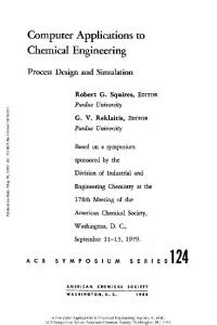
Macroblock-Level Parallelism

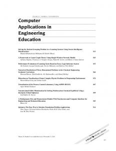
To exploit parallelism between macroblocks (MBs) it is necessary to take into account the dependencies between them. In H.264, motion vector prediction, intra prediction, and the deblocking filter use data from left, upper-left, upperright, and upper neighboring MBs. MBs can be processed out of scan order provided these dependencies are satisfied. Processing MBs in a diagonal wavefront manner satisfies all the dependencies and therefore allows to exploit parallelism between MBs. We refer to this parallelization technique as 2D-Wave, to distinguish it from the 3D-Wave proposed in this chapter. Figure 2.5 depicts an example for a 5×5 MBs image frame (80×80 pixels). Assuming it takes one time slot to decode a MB, at time slot T7 three independent MBs can be processed: MB (4,1), MB (2,2), and MB (0,3). The figure also shows the dependencies that need to be satisfied in order to process each of these MBs. The maximum number of independent MBs in a frame depends on the resolution. Figure 2.6 depicts the available MB-level parallelism over time for Standard Definition (SD), High Definition (HD), and Full High Definition (FHD) resolutions, assuming that the time to decode a MB is constant. In other words, it shows the number of MBs that can be decoded in parallel at each time slot.

22


FOR

H.264...

FHD HD SD

60

Parallel macroblocks

50

40

30

20

10

0 0

50

100

150

200

250

Time

Figure 2.6: MB parallelism for a single SD, HD, and FHD frame using the 2D-Wave approach.

MB-level parallelism has several advantages over other parallelization schemes for H.264. First, this scheme potentially has good scalability since, as shown in Figure 2.6, the number of independent MBs increases with the resolution of the image. Second, it is possible to achieve good load balancing provided a dynamic scheduling system is used. A dynamic scheduling system is a system that dynamicaly evaluates dependency resolutions and is needed because the time to decode a MB is not constant and depends on the data being processed. The load would be balanced if a centralized scheduler would dynamically assign a MB to a processor once all the dependencies of the MB have been satisfied. Additionally, because in MB-level parallelization all the processors/threads run the same program, the same set of software optimizations (for exploiting ILP and SIMD) can be applied to all processing elements. MB-level parallelism has also some disadvantages, however. The first one is that the entropy decoding cannot be parallelized using data decomposition, due to the fact that the lowest level of data that can be parsed from the bitstream are slices. Individual MBs cannot be identified without performing entropy decoding. That means that in order to decode independent MBs, they should be entropy decoded first, in sequential order. This disadvantage can be overcome by using special purpose instructions or hardware accelerators for the entropy decoding process, such as the hardware accelerator described in [75].

2.4. 3D-WAVE S TRATEGY

23

The second disadvantage is that the number of independent MBs does not remain constant during the decoding of a frame, as can be seen in Figure 2.6. Therefore, it is not possible to sustain a certain processing rate during the decoding of a frame. This problem is solved by using the parallelization strategy proposed in Section 2.4. MB-level parallelism has been proposed in previous work. Van der Tol et al. [95] proposed the exploitation of MB-level parallelism for optimizing the H.264 decoding. The analysis was performed for a multiprocessor system consisting of 8 Trimedia processors with private L1 caches and a shared L2 cache. The paper also suggested the combination of MB-level with frame-level parallelism to increase the number of independent MBs, but did not analyze it thoughtfully. The use of frame-level parallelism is determined statically by the length of the MVs. Chen et al. [20] evaluated a similar approach for a H.264 encoder: a combination of MB- frame-level parallelism on Pentium machines with SMT and CMP capabilities. In the above mentioned works the exploitation of frame-level parallelism is limited to two consecutive frames and the identification of independent MBs is done statically by taking into account the maximum allowed MV length, which is roughly half the vertical resolution of the frame. 2.3.2.5

Block-Level Parallelism

The finest grain of data-level parallelism is at the block level. Most computations of the H.264 basic modules are performed at the block level. This applies, for example, to the interpolations performed at the motion compensation stage, to the IDCT, and to the deblocking filter. This level of data parallelism maps well to SIMD instructions [104, 90, 5, 56]. SIMD parallelism is orthogonal to the other levels of parallelism described above and because of that it can be combined, for example, with MB- and frame-level parallelism to increase the performance of each thread.

2.4 3D-Wave Strategy None of the approaches described above scale to future many-core architectures consisting of 100 cores or more. Figure 2.6 shows that in the 2D-Wave, there is a considerable amount of MB-level parallelism, but at the beginning and at the end of processing a frame, there are only a few MBs that can be processed in parallel. In this work we propose to start decoding a MB as soon

24


FOR

H.264...

as its reference area in the reference frame has been decoded. In other words, we combine MB-level parallelism with frame-level parallelism. We refer to our strategy as the 3D-Wave.

2.4.1 Parallelization Strategy In the decoding process there are dependencies between frames only in the Motion Compensation (MC) module. MC can be regarded as copying an area, called the reference area, from the reference frame, and then adding this predicted area to the residual MB to reconstruct the MB in the current frame. The reference area is pointed to by a Motion Vector (MV). The MV length is limited by two factors: the H.264 level and the motion estimation algorithm. The H.264 standard has levels which define the maximum length of the vertical component of the MV and a fixed horizontal component for all levels from -2048 to 2047.75, inclusive [2]. In the encoding process the motion estimation maximum search range is usually restricted to only dozens of pixels, because increasing the search range is very computationally demanding and provides only a small benefit [61]. Most motion estimation algorithms use some kind of strategy to decrease the search area, since exhaustive searching the full range is computationally too expensive. When the reference area has been decoded it can be used by the referencing frame. Thus it is not necessary to wait until the entire frame, or maximum reference area, is completely decoded before decoding the next frame, as in Van der Tol et al. [95]. The decoding process of the next frame can start after the reference area of the reference frame(s) has been decoded. Figure 2.7 illustrates the 3D-Wave parallel decoding of frames, each of which is decoded using the 2D-Wave strategy.

2.4.2 3D-Wave Static Evaluation In order to obtain a first approximation of the potential of combining MBlevel parallelism with frame-level parallelism, we developed a static analysis method. This method computes the number of MBs that could be processed in parallel when decoding a video sequence, for a given MV range. In this analysis a MB can be decoded after its reference range has been decoded in the reference frame and its intra-frame dependencies has been satisfied. Figure 2.8 illustrates the reference range concept, assuming a MV range of 32 pixels. The hashed MB in Frame 1 is the MB under consideration. Its reference range is


25

Figure 2.7: 3D-Wave strategy: Frames can be decoded partially in parallel because inter-frame dependencies have a limited range.

Figure 2.8: Reference range example: The hashed area in Frame 0 is the reference range of the hashed MB in Frame 1.

represented by the hashed area in Frame 0. The MV can point to any area a the range of [-32,+32] pixels, representing an offset in the vertical and horizontal directions from the MB under consideration. In the same way, every MB in the wavefront of Frame 1 has a reference range similar to the presented one, with its respective displacement. In this analysis, we assume that all available MBs are processed in parallel and have the same processing time. Once the reference range of the first (upper-left) MB is decoded, the 2D-Wave decoding of the frame can start. In this analysis the following conservative assumptions are made to calculate the amount of MB-level parallelism. First, B frames are used as reference frames, since in the H.264 standard, B frames can be used as reference frames. This also makes the evaluation valid for the Baseline profile of the standard, where B frames are not used. When B frames are not used as refer-

26


FOR

H.264...

ence frames they can be decoded in parallel with other B frames and with the next P frame in the decoding order. Second, the reference frame is always the previous one. H.264 allows multiple reference frames. In this evaluation the worst case is assumed, since having the previous frame as the reference frame limits the progression of the wave decoding of the current frame. In other words, the older the reference frame is, the further it has been decoded. Third, only the first frame of the sequence is an I frame. As I frames do not have inter frame dependencies, they can be decoded in parallel with their preceding frames. The number of frames between I frames, however, is defined by the encoder and can be arbitrary large, e.g., 60 frames or more. Because of that, only the first frame of the video sequence is considered to be an I frame. The static analysis methodology of the 3D-Wave strategy can be described as follows: Given a MV range, it is possible to determine the number of time steps that have to elapse between the decoding of two consecutive frames. For example, for MVs with a maximum length of 16 pixels, it is possible to start the decoding of the second frame when the MBs (0,0), (0,1), (1,0), and (1,1) of the first frame have been decoded. Of these MBs, (1,1) is the last one decoded in 2D-Wave order, namely at time t = 3. So when the maximum MV length is 16 pixels, we can start decoding the second frame at time t = 4, and the third frame at time t = 8, etc. Similarly, we find that for a maximum MV length of 32 pixels, we can start decoding the second frame at time t = 7 and the third frame at time t = 14. For maximum MV lengths of 64, 128, 256, and 512, we can start decoding the second frame at time t = 13, 25, 49, and 97, respectively. In general, for a MV range length of n pixels (⌈n/16⌉ MBs), the decoding of the second frame can start at time t = 1 + 3 × ⌈n/16⌉. The number of parallel MBs available in a video sequence is calculated based on the overlap between consecutive frames (each one decoded using the 2D-Wave). The number of available parallel MBs in each time step. Let N2D (t) be the number of parallel MBs at time step t using the 2D-Wave. Then the number of parallel MBs N3D (t) at time step t of the 3D-Wave is given by X

t/of f set

N3D (t) =

N2D (t − i × of f set)

(2.1)

i=0

where of f set is the number of time steps that have to elapse between the decoding of two consecutive frames.

2.4. 3D-WAVE S TRATEGY 400

Frame 9 Frame 8 Frame 7 Frame 6 Frame 5 Frame 4 Frame 3 Frame 2 Frame 1 Frame 0

350

300


27

250

200

150

100

50

0 0

20

40

60

80

100

120

140

Time

Figure 2.9: Stacking of frames of a FHD sequence with a 128 pixels maximum MV length.

Figure 2.9 depicts this function for the first 10 frames of a FHD sequence with a maximum MV length of 128 pixels. It also shows to which frame each MB belongs. It can be seen that a stacking effect occurs. The videos from HD-VideoBench [7] benchmark was chosen because of their resolution and the content of the scenes. The benchmark contains the following test sequences: • rush hour: rush-hour in Munich city; static background, slowly moving objects. • riverbed: riverbed seen through waving water; abrupt and stochastic changes. • pedestrian area: shot of a pedestrian area in city center; static background, fast moving objects. • blue sky: top of two trees against blue sky; static objects, sliding camera. All movies are available in three formats: 720×576 (SD), 1280×720 (HD), 1920×1088 (FHD). Each movie has a frame rate of 25 frames per second and has a length of 100 frames.

28


FOR

H.264...

Table 2.1: Static 3D-Wave results of available parallel MBs and number of frames in flight.

Offset 512 256 128 64 32 16 2.4.2.1

Max # Parallel MBs SD HD FHD 40 91 34 76 169 66 145 328 126 277 629 232 515 1166 414 900 2040

Max # Frames in Flight SD HD FHD 2 3 3 4 6 5 7 11 9 13 20 17 24 37 29 42 64

Maximum Parallelism

Using the static analysis we determined the number of parallel MBs in the 3D-Wave for each video resolution in the HD-VideoBench, SD, HD, and FHD with MV ranges of 16, 32, 64, 128, 256, and 512 pixels. 512 pixels is the maximum vertical MV length allowed for level 4.0 in the H.264 standard. Figure 2.10 depicts the MB-level parallelism (i.e., the number of MBs that can be processed in parallel) obtained by the static analysis of the 3D-Wave strategy for each point in time for an FHD sequence using different maximum MVs ranges. The results show that the 3D-Wave strategy is much more scalable than the 2D-Wave strategy. For example, while the 2D approach can process at most 60 MBs in parallel for FHD resolution, the 3D-Wave strategy achieves 1150 parallel MBs for a MV range of 32 pixels and more than 2000 parallel MBs for a MV range of 16 pixels. Furthermore, the 3D-Wave strategy can process more than 80 MBs in parallel even when the MV range is 512 pixels (almost half the frame height). An additional advantage of the 3D-Wave is that after a certain time, the number of parallel MBs stays constantly high. This is in contrast to the 2D-Wave strategy, which achieves little parallelism at the beginning and at the end of processing each frame. Figure 2.11 depicts the number of frames in flight for different MV ranges. The time unit is the time required to process one MB (which is assumed to be constant in this evaluation). The shapes of the SD and HD resolutions curves are similar and are therefore not presented for brevity. Instead, Table 2.1 presents the maximum MB parallelism and number of frames in flight for SD, HD and FHD video sequences.


29

MV 16 MV 32 MV 64 MV 128 MV 256 MV 512

2000


1500

1000

500

0 0

100

200

300

400 Time

500

600

700

Figure 2.10: Number of parallel MBs in the 3D-Wave for FHD frames with different MV ranges.

MV 16 MV 32 MV 64 MV 128 MV 256 MV 512

60

Frames in flight

50

40

30

20

10

0 0

100

200

300

400 Time

500

600

700

Figure 2.11: Frames in flight for FHD frames with different MV ranges.

30


FOR

H.264...

2.5 Limited Resources A potential problem of the 3D-Wave strategy is, however, the large number of frames that are decoded simultaneously. Figure 2.11 depicts the number of frames in flight at each point in time for an FHD sequence and different MV ranges. The figure shows that when, for example, the MV range is 16 pixels, there can be up to 64 frames in flight simultaneously. This can be a problem in systems with limited memory since each active frame has to be stored in memory. To investigate this limitation, we have also analyzed the tradeoff between the number of active frames and the amount of MB-level parallelism. In this analysis the number of active frames is limited. The decoding of the next frame is started only if the number of active frames is less than or equal to a specified maximum number of frames in flight. If this is not the case, the decoding of the next frame has to wait until a frame is decoded. The analysis focuses on FHD resolution with a MV range of 16 pixels. This MV range has been chosen because it clearly shows the effect of limiting the number of frames in flight, as it has the maximum amount of MB-level parallelism. The maximum number of frames in flight was set to 4, 8, 16, and 32. Figure 2.12 presents the results. For reference, the curve for the case that does not limit the number of active frames is also shown. Limiting the number of frames in flight has two different effects on the amount of MB-level parallelism. The first one is a proportional decrease of the average number of parallel MBs. After the ramp up part of the MB parallelism curve, there are 2040 MBs available when there is no limit on the number of frames in flight in which case there are up to 64 frames in flight. Limiting the number of active frames to 32, the average number of MBs available to be processed in parallel is reduced to 1020. For 16, 8, and 4 active frames, the results show an average of 508, 253, and 126 parallel MBs, respectively. The second effect of limiting the number of frames in flight is that the number of parallel MBs fluctuates over time, as can be seen in Figure 2.12. While there is just a very small (or no) fluctuation when there is no limit on the number of active frames, the fluctuation is large when the number of active frames is limited. This fluctuation also increases when the number of active frames decreases. For 32 active frames, after the ramp up, at most 1528 and at least 512 parallel MBs are available. Limiting the number of active frames to 16, 8, and 4, the maximum number of available MBs becomes 888, 472, 240 and the minimum is 128, 32, 8 MBs, respectively. This fluctuation is the result of the superposition of peaks in the 2D-Wave MB parallelism curves.

2.5. L IMITED R ESOURCES

31

Unlimited 32 16 8 4

2000


1500

1000

500

0 0

100

200

300

400 Time

500

600

700

Figure 2.12: Macroblock parallelism with limited frames in flight.

The fluctuation of the number of available parallel MBs can result in underutilization of computational resources. This can happen, for instance, when the number of cores available is larger than the number of available parallel MBs at a given time. A scheduling technique can be used to reduce the fluctuation of the amount of MB-level parallelism. To minimize the fluctuation, we should start decoding the next frame Tframe /nactive time units after the time we have started decoding the current frame, where Tframe is the processing time of a frame and nactive is the maximum number of active frames. Figure 2.13 shows the curves resulting from this scheduling strategy. This strategy has a small effect on the average amount of MB-level parallelism, compared with limiting the frame parallelism without the scheduling. Table 2.2 presents the maximum, minimum, and average MB parallelism with and without scheduling. As can be seen in this table, the amount of MB-level parallelism is proportional to the number of allowed frames in parallel.

32


FOR

H.264...

Unlimited 32 16 8 4

2000


1500

1000

500

0 0

100

200

300

400 Time

500

600

700

Figure 2.13: Scheduled macroblock parallelism with limited frames in flight.

Table 2.2: Number of available parallel MBs with and without the proposed scheduling technique, for FHD.

Frames in Flight 32 16 8 4

Max 1528 888 472 240

Min 512 128 32 8

Regular Fluctuation 66% 86% 93% 97%

Avg 1020 508 252 124

Max 1148 544 264 127

With Scheduling Min Fluctuation 872 24% 484 11% 202 23% 67 47%

Avg 1010 514 233 97

2.6. DYNAMIC 3D-WAVE

33

2.6 Dynamic Analysis of the 3D-Wave ‡ In the previous section we have analyzed the 3D-Wave using a static approach, considering that the MV length of all MBs is equal to a given maximum. In reality, however, the MV length of each MB may differ. For completeness and because the implementation described in the next chapter have similar behavior, in this section we briefly present a dynamic analysis of the 3D-Wave. Meenderinck et al. [66] evaluate the 3D-Wave technique using a dynamic approach. This dynamic approach computes the number of available parallel MBs considering their actual dependencies in the evaluated video sequence. As before, it is assumed that it takes one time unit to decode a MB. To determine the amount of parallelism, the FFmpeg H.264 decoder [37] was modified to analyze the MB dependencies in real video sequences. Each MB has its dependencies analyzed and a timestamp assigned as follows. The timestamp of a MB is simply the maximum of the timestamps of all MBs upon which it depends (in the same frame as well as in the reference frames) plus one. Because the frames are processed in decoding order, and within a frame the MBs are processed from left to right and from top to bottom, the MB dependencies are observed and it is assured that the MBs on which a MB B depends have been assigned their correct timestamps by the time the timestamp of MB B is calculated. The video sequences are from the HD-VideoBench. However, because the sequences have only 100 frames, the used input sequences are composed of the original sequences replicated four times. The encoding is performed by the X264 encoder using the following options: 2 B-frames between I and P frames (B frames cannot be reference frames), 16 reference frames, weighted prediction, hexagonal motion estimation algorithm (hex) with a maximum search range of 24, one slice per frame, and adaptive block size transform. Movies encoded with this set of options represent the typical case. Figure 2.14 depicts the MB-level parallelism time curve for FHD, while Figure 2.15 depicts the number of frames in flight in each time slot. The results show peaks of 4.000 to 7.000 parallel MBs. The maximum number of frames in flight is just above 200 for all sequences. These results show that much more parallelism is available in actual video sequences than indicated by the static analysis. For example, the static analysis reported a maximum of 2.040 parallel MBs for a FHD sequence while the dynamic analysis reports between 2.000 to 4.000 parallel MBs, after ramp‡

This section is based on work performed by Cor Meenderinck.

34

C HAPTER 2. A S CALABLE PARALLEL A LGORITHM 8000

FOR

H.264...

rush_hour riverbed pedestrian blue_sky

7000


6000

5000

4000

3000

2000

1000

0 0

200

400

600 Time

800

1000

1200

Figure 2.14: Number of parallel MBs in each time slot for the 3D-Wave, using the dynamic analysis, for FHD resolution using a 400-frame sequence.

up, for the pedestrian sequence, which is the sequence with the lowest number of parallel MBs among the tested sequences. This is due to two factors. First, the static evaluation only considers inter-dependent frames while the dynamic evaluation uses 2 B frames between P frames. As the 2 B frames are independent from each other, they can be processed in parallel as well as the next P frame. This is a three fold increase in the number of MBs and frames in parallel. Second, the smallest range for the static evaluation considers a maximum MV length of 16 pixels, while the average MV length in the evaluated sequences for the dynamic evaluation is about 5 pixels. As reported in the previous section, the number of parallel MB increases when the MV length decreases. This study adds more precision to the static analysis presented earlier and confirms our findings. However, it still presents limitations. The MB decoding time is assumed to be fixed while in reality this is not the case. By itself this reduces the available MB parallelism by 33% [3]. Another limitation is that our analysis does not include the synchronization overhead. Synchronization overhead can be a major problem in a parallel implementation of the decoder [4]. Moreover, an implementation mechanism is not proposed. These limitations will be addressed in our implementation of the 3D-Wave on a many-core processor in the next chapter.

2.7. C ONCLUSIONS

35

250

rush_hour riverbed pedestrian blue_sky

Frames in flight

200

150

100

50

0 0

200

400

600 Time

800

1000

1200

Figure 2.15: Number of frames in flight in each time slot for the 3D-Wave, using the dynamic analysis, for FHD resolution using a 400-frame sequence.

2.7 Conclusions In this chapter we have investigated if contemporary and perhaps future video applications exhibit sufficient parallelism to exploit the large number of cores expected in future many-core processors. As a case study, we have analyzed the parallel scalability of the H.264 video decoder, currently the leading video coding standard. First, we have discussed different ways to parallelize H.264 and showed that slice-level parallelism has two main limitations. First, using many slices increases the bitrate and, second, not all sequences contain sufficient slices to scale to a large number of cores, since the encoder determines the number of slices per frame. It was also shown that frame-level parallelism, which exploits the fact that some frames (B frames) are not used as reference frames and can therefore be processed in parallel, is also not very scalable, because usually there are no more than three B frames between consecutive P frames and, furthermore, in H.264 B frames can be used as reference frames. More promising is MB-level parallelism, which can be exploited inside a frame in a diagonal wavefront manner. Intra-frame MB-level parallelism, however, exhibits at most 60 parallel MBs, which is not sufficient for a manycore. It was observed that MBs in different frames are only dependent through MVs which have a limited range. We therefore proposed a novel parallelization strategy, called 3D-Wave, which combines MB-level parallelism with frame-

36


FOR

H.264...

level parallelism. The MB-level parallelism available in the 3D-Wave was analyzed using a static and a dynamic approach. In the static approach, for FHD resolution, the results show that when the MV range is limited to 16 pixels, up to 2040 MBs can be processed in parallel. In the worst case, when the MV is at most 512 pixels, at most 91 parallel MBs are available, which is still much more than the number of parallel MBs other parallelization approaches reach. Furthermore, we showed that the fluctuation of the number of parallel MBs can be reduced by applying a simple scheduling strategy. Nevertheless, this static analysis is conservative since it is based on the assumption that the MV length of each MB is equal to the maximum MV length. A dynamic evaluation of the 3D-Wave showed that in real video sequences with regular coding options, there is even more MB-level parallelism than the static evaluation suggests.

3 3D-Wave Implementation

I

n the previous chapter we have proposed the 3D-Wave parallelization strategy for H.264 video decoding. It has been shown that the 3D-Wave strategy potentially scales to a much larger number of cores than previous strategies do. However, we have done so using a very high-level evaluation methodology, assuming constant macroblock (MB) decoding time and zero communication and synchronization overhead. In this chapter we remedy these limitations by presenting an implementation of 3D-Wave parallelization strategy on an embedded many-core with up to 64 cores. This chapter is organized as follows. Section 3.1 motivates the presented implementation and details the contributions of this chapter. In Section 3.2 the simulation environment and the experimental methodology used to evaluate the proposed 3D-Wave implementation are presented. In Section 3.3 the implementation of the 3D-Wave on the embedded many-core is detailed. This section also presents a frame scheduling policy used to limit the number of frames in flight and the priority policy used to reduce latency. Additionally, a 3D-Wave visualization tool is also described in Section 3.3. Section 3.4 presents extensive experimental results analyzing the following aspects: scalability and performance of the 3D-Wave, the policies for frame scheduling and priority, the impacts of the memory latency, L1 cache size, parallelization overhead, and entropy decoding. Conclusions are drawn in Section 3.5.

37

38

C HAPTER 3. 3D-WAVE I MPLEMENTATION

3.1 Introduction In the previous chapter we have proposed the 3D-Wave parallelization strategy for H.264 video decoding. It has been shown to potentially scale to a much larger number of cores than existing strategies do. However, the previous chapter presented only analytical results. It analyzed how many macroblocks could be processed in parallel assuming infinite resources, no communication delay, infinite bandwidth, and a constant MB decoding time. In this chapter we present an implementation of the 3D-Wave strategy on an embedded many-core consisting of up to 64 cores. Implementing the 3D-Wave turned out to be quite challenging. First, it requires to dynamically identify inter-frame MB dependencies and handle their thread synchronization, in addition to intra-frame dependencies and synchronization. In our previous analytical analysis thread synchronization was not an issue because the MBs were visited sequentially and assigned a timestamp representing the earliest time slot in which they could be processed. For the 3D-Wave strategy both intra- and inter-frame synchronization have to be taken into account in a way that the synchronization overhead does not limit the scalability, for the target number of cores. This led to the development of a subscription mechanism where the current MB checks if the MBs it depends on are already processed. If one of the MBs is not yet processed, the current MB subscribes itself to a so-called Kick-off List (KoL) associated with the MB it depend on and halts. The processing of halted MBs is restarted when the current MB, after finishing its processing, resumes the processing of MBs subscribed to its KoL. A potential drawback of the 3D-Wave strategy is that the decoder latency may become unbounded because many frames are decoded simultaneously. A policy is presented that gives priority to the oldest frame so that newer frames are only decoded when there are idle cores. Another potential drawback of the 3D-Wave strategy is that the memory requirements might increase because of the large number of frames in flight. To overcome this drawback we present a frame scheduling policy to control the number of frames in flight. The effect of memory system, thread synchronization, and entropy decoding in the 3D-Wave scalability are also analyzed in this Chapter. Memory requirements are an issue when dealing with parallel applications. We analyze the impact of the memory latency and the L1 cache size on the scalability and performance of the 3D-Wave strategy. The experimental platform features hardware support for thread management and synchronization, making it relatively light weight to submit/retrieve a task to/from a task pool. We analyze the

3.2. E XPERIMENTAL M ETHODOLOGY

39

importance of this hardware support by artificially increasing the time it takes to submit/retrieve a task. The 3D-Wave focuses on the MB decoding part of the H.264 decoding and assumes an accelerator for entropy decoding. Finally, we analyze the performance required from the entropy decoding accelerator to avoid affecting the 3D-Wave scalability.

3.2 Experimental Methodology In this section the tools and methodology used to implement and evaluate the 3D-Wave technique are detailed. The components of the many-core system simulator used to evaluate the technique are also presented. An NXP proprietary simulator based on SystemC is used to run the application and collect performance data. Computations on the cores are modeled cycle-accurate. The memory system is modeled using average transfer times with channel and bank contention. When channel or bank contention is detected, the traffic latency is increased. NoC contention is also modeled. The simulator is capable of simulating systems with up to 64 TM3270 [94] cores with shared memory and their cache coherence protocol. The operating system is not simulated. The TM3270 is a Very Large Instruction Word (VLIW) mediaprocessor based on the Trimedia architecture. It is targeted at the requirements of multi-standard video processing at standard resolution and the associated audio processing requirements for the consumer market. The architecture supports VLIW instructions with five guarded issue slots. The pipeline depth varies from 7 to 12 stages. Address and data words are 32 bits wide. The unified register file has 128 32-bit registers. 2×16-bit and 4×8-bit SIMD instructions are supported. To produce code for the TM3270 the state-of-the-art highly optimizing NXP TriMedia C/C++ compiler version 5.1 is used. For our experiments, the TM3270 processor clock frequency was set to 300 MHz. The modeled system features a shared memory using the MESI cache coherence protocol. Each core has a private L1 data cache and can copy data from other L1 caches through 4 channels. The 64KB L1 data cache has 64-byte lines and is 4-way set-associative with LRU replacement and write allocate policies. The instruction cache is not modeled. It is not considered to be a limitation because as the code is concise and highly optimized, it would fit in a regular sized instruction cache. The cores share a distributed L2 cache with 8 banks and an average access time of 40 cycles. The average access time takes into account L2 hits, misses, and interconnect delays. L2 bank

40


contention is modeled in the simulator, thus two cores cannot access the same bank simultaneously. The multi-core programming model follows a task pool model. A Task Pool (TP) library implements submissions and requests of tasks to/from the task pool, synchronization mechanisms, and the task pool itself. Each core runs a thread by requesting a task from the TP, executing it, possibly identifying and submitting tasks to the TP, and requesting another task. The task execution overhead is low. The time to request a task is less than 2% of the MB decoding time. The experiments focus on the baseline profile of the H.264 standard. This profile only supports I and P frames and every frame can be used as a reference frame. This feature prevents the exploitation of frame-level parallelization techniques such as the one described in [20]. This profile, however, highlights the advantages of the 3D-Wave, since the scalability gains come purely from the application of the 3D-Wave technique. Encoding was done with the X264 encoder [102] using the following options: no B-frames, at most 16 reference frames, weighted prediction, hexagonal motion estimation algorithm with a maximum search range of 24, and one slice per frame. The experiments use all four videos from the HD-VideoBench [7]. The 3D-Wave technique focuses on the TLP available in the MB processing kernels of the decoder. The entropy decoder is known to be challenging to parallelize. To isolate the influence of the entropy decoder, its output has been buffered and its decoding time is not taken into account. Although it is not the main objective, as a side effect the 3D-Wave also eases the entropy decoding challenge. Since entropy decoding dependencies do not cross slice/frame borders, multiple entropy decoders can be used. We analyze the performance required from an entropy decoder accelerator in Section 3.4.7.

3.3 Implementation Our work is based on the NXP H.264 decoder. The 2D-Wave parallelization strategy has already been implemented in this decoder [46], making it a perfect starting point for the implementation of the 3D-Wave. The NXP H.264 decoder is highly optimized, including both machine-dependent optimizations (e.g. SIMD operations) and machine-independent optimizations (e.g. code restructuring).

3.3. I MPLEMENTATION

41

The 3D-Wave implementation serves as a proof of concept and thus the implementation of all features of H.264 is not necessary. Intra prediction inputs are deblock filtered samples instead of unfiltered samples as specified in the standard. This does not, however, add perceptive visual artifacts to the decoded frames or change the MB dependencies. This section describes the 2D-Wave implementation used as the starting point, the 3D-Wave implementation, and the frame scheduling and priority policies.

3.3.1 2D-Wave Implementation The MB processing tasks of the 2D-Wave implementation consists of four kernels that are grouped slightly different than previously presented. The kernels are vector prediction (VP), picture prediction (PP), deblocking info (DI), and deblocking filter (DF). VP calculates the motion vectors (MVs) based on the predicted motion vectors of the neighbor MBs and the differential motion vector present in the bitstream. PP performs the reconstruction of the MB based on neighboring pixel information (Intra Prediction) or on reference frame areas (Motion Compensation). Inverse quantization and the inverse DCT are also part of this kernel. DI calculates the strength of the DF based on MB data, such as the MBs type and MVs. Finally, DF smooths block edges to reduce blocking artifacts. Each kernel is parallelized using the 2D-Wave strategy. As shown in Figure 2.5 on page 21, within a frame each MB depends on at most four other MBs. These dependencies are covered by the dependencies from the left MB to the current MB and from the upper-right MB to the current MB. In other words, if the left and the upper-right dependencies are satisfied then all dependencies are satisfied. Therefore, in the implementation each MB is associated with a reference count between 0 and 2 representing the number of MBs it depends on. For example, the upper-left MB has a reference count of 0, the other MBs at the top edge and at the left edge have a reference count of 1. When a MB has been processed, the reference counts of the MBs that depend on it are decremented. When one of these counts reaches zero, a thread that will process the associated MB is submitted to the TP. Figure 3.1 depicts pseudo C-code for applying the DF on a frame and on a MB. tp_atomic_decrement atomically decrements the counter and returns its value. tp_submit submits a function and its parameters to the TP.

42


int deblock_ready[w][h]; // matrix of reference counts void deblock_frame() { for (x=0; x 3; p1’ = (p2 + p1 + p0 + q0 + 2) >> 2; p2’ = (2*p3 + 3*p2 + p1 + p0 + q0 + 4) >> 3; } else p0’ = (2*p1 + p0 + q1 + 2) >> 2; } else p0’ = (2*p1 + p0 + q1 + 2) >> 2;

Figure 4.5: Filtering function for Intra MB boundaries.

clip(x, y, z){ return x < y ? y : ( x > z ? z : x) } clip(x) {return clip(x, 0, 255)} if( p2 - p0 < beta){ p1’’ = ((p2 + ((p0 + q0 + 1) >> 1)) >> 1) - p1; p1’ = p1 + clip(p1’’, -tc0, tc0); } delta’ = delta = p0’ =

(((q0 - p0 ) >3; clip(delta’,-tc, tc); clip( p0 + delta );

Figure 4.6: Filtering function for other MB boundaries.

75

76

C HAPTER 4. S UITABILITY

OF

SIMD-O NLY C ORES

FOR

K ERNELS ...

4.5 Implementation In this section, the implementation of the DF on the Cell SPE is detailed. The implementation will be described in a top-down fashion starting with the main loop of the kernel and gradually goes down to the inner parts of the implementation. The focus of this analysis is the computational part of the DF. The baseline version is a scalar implementation extracted from the FFMPEG H.264 decoder [37]. The extracted code does not include the parameter calculation of the DF. The analysis focuses on the sample filtering of the code. This scalar version is then vectorized using the SIMD intrinsics for the SPE and AltiVec intrinsics for the PPE. Because the AltiVec implementation is very similar to the SPE version, only the SPE version will be presented. In the SPE implementations, the PPE is used only to read the parameters from the input files and to store them in main memory. After storing the parameters, the SPE threads are spawned. Thereafter, the PPE thread sends a signal to all SPEs to start the computation. Each SPE thread processes one frame. The 3D-Wave technique was not considered because this research was performed before the 3D-Wave technique was developed. The processing of the DF per frame, however, avoids data movements between SPEs and/or between SPEs and main memory as all data dependencies are between instructions executed on the same SPE. The processing starts by reading the input pointers for the samples and parameters from the main memory. Each frame is divided into several MB lines (MBs from the same row), in order to use the SPE’s ability of performing computation and data communication in parallel. This partitioning is based on several factors such as the latency, maximum DMA transmission package size, number of DMA transfers, and organization of the data in the memory. The start-up latency increases with the partition size, so a large partition incurs large start-up latency. The pixel components Y, Cb, and Cr are stored in separate arrays. Partitioning into complete lines of MBs allows to load the pixel samples of one partition with three DMA transfers. Using partitions that do not cover complete lines would require a separated DMA request for each pixel line in the partition. For every MB line there are four DMA transfers from memory to the LS. One DMA transfer is necessary for 16 lines of luma samples, two for 8 lines of each set of chroma samples, and another one for the DF parameters of the MB line. After the data is available in the LS, the processing of the MB line is performed and the results are transmitted back to the main memory.

4.5. I MPLEMENTATION

DMA.get

77

(MB_Line[0]);

DMA.get (MB_Line[1]); DMA.wait (MB_Line[0]); Filter (MB_Line[0]); FOR x = 2 TO { DMA.get DMA.wait Filter DMA.put }

frame_height_in_MB -1 (MB_Line[x]); (MB_Line[x-1]); (MB_Line[x-1]); (MB_Line[x-2]);

Filter DMA.put

(MB_Line[x-1]); (MB_Line[x-2]);

DMA.put

(MB_Line[x-1]);

Figure 4.7: Double buffering of MB lines.

Figure 4.8: Deblocking Filter processing diagram.

The processing of the MB lines is performed as a software pipeline and uses a double buffering strategy. First, the data for the first MB line is requested, followed by the request of the data for the second MB line. After the data of the first MB line is available in the LS, it is filtered. This way the processing of MB line i is performed in parallel with the DMA transfer of of MB line i+1 from memory to the LS. The pseudo-code in Figure 4.7 illustrates the process. Figure 4.8 depicts the diagram of the DF process. The gray area in Filter indicates the waiting time for the DMA request to complete. The processed MB line cannot be immediately transmitted back to memory. As depicted in Figure 4.4, the processing of the next MB line changes the values of the current bottom edge samples.

78


OF

SIMD-O NLY C ORES

FOR

K ERNELS ...

The filter process is performed per MB. As described in Section 4.4, there are 8 edges, four vertical and four horizontal. First the four vertical edges are filtered and then the four horizontal. The filtering process is divided into the following steps: (1) unpack the 8-bit (8b) samples of the current and left MBs to signed 16b, (2) transpose the current and left MBs so the pixels to be filtered are moved from inside the same quadword (as in Figure 4.3(a)) to different quadwords, and thus, more amenable to SIMD processing, (3) filter the vertical edges, (4) transpose the result, (5) pack back the left MB result to 8b, (6) unpack the last 4 lines of the top MB to 16b, (7) filter the horizontal edges, and finally, (8) pack back the MB result to 8b. The computational core of the DF is the edge filtering. There are four functions required to implement the edge filtering. Luma and chroma samples require two functions each: one for Intra MB external edges blocks and another one for the other cases. These functions exhibit data-level parallelism and have been optimized with SIMD instructions of the SPE, such that the edge filtering computes 8 pixels simultaneously. Because of the high branch penalties, it is necessary to eliminate branches whenever possible to improve performance. To perform the filtering without branches, all equations of the function have to be computed. All branches are replaced by comparisons that result in a mask. These masks are used to select the positions of the result vectors that will be written back to memory. All the filtering functions have been implemented without branches, except for the one to select between the filter processes listed above. The impact on the performance of the SIMD-only core is analyzed in the next section.

4.6 Experimental Results In this section, the experimental results are presented. First, the input data and methodology are described. It is followed by an analysis of the results. Based on the analysis, the conclusions are drawn. As input, the first eight frames of the Lake Wave video sequence, in the QVGA (320×240 pixels) resolution, are used. The reason why we used a QVGA video sequence is that at the time of this research was performed, only QVGA sequences were available to us. Furthermore, the goal was to compare a SIMD implementation to a scalar one and for this, the QVGA resolution is sufficient. The time is measured using the SPE hardware counters. The presented results are the average of three runs.

4.6. E XPERIMENTAL R ESULTS

79

Figure 4.9 depicts the time in milliseconds required to filter a single frame for each version of the kernel: the scalar version running on the PPE (PPE - Scalar), the AltiVec version on the PPE (PPE - AltiVec), the scalar version on the SPE (SPE - Scalar), the SIMD version on the SPE without double buffering (SPE - SIMD no D.B.), and the SIMD version on the SPE with double buffering (SPE - SIMD D.B.). For the scalar versions, filtering a QVGA frame takes on average 2.79 and 2.72 ms on the PPE and SPE, respectively. The PPE AltiVec implementation has an average run-time of 2.15 ms, which is 30% faster than the PPE scalar version. The SPE SIMD version takes 1.14 ms per frame, while using a double buffering technique reduces the average runtime to 1.05 ms. The latter corresponds to a speedup of 2.6 compared to the SPE scalar version. For comparison, SIMD implementations of the DF for SSE2 have been presented in [57, 97] where speedups of 1.13 and 1.49 respectively, are reported. As the AltiVec and SPE SIMD versions are almost identical, the difference in speedup obtained by vectorizing with SIMD instructions is interesting. A critical difference between the PPE AltiVec unit and the SPE is that the first one has only 32 vector registers, while the second has 128. Profiling the SPESIMD version using the IBM Cell Full-System Simulator [17] showed that all 128 registers are used, with an average of 120 registers alive. Because a MB is much larger than the PPE AltiVec register file, additional loads/stores are required, decreasing performance. Moreover, the SPE versions benefit from the LS, since no cache conflicts occur, and the direct access to main memory through the DMAs, as the kernel has a predefined memory access pattern. The performance difference between the double buffering implementation with the non-double buffering is only 8%. The profiling results also show that the double buffering strategy successfully hides the communication latency. The total number of cycles the cores are stalled waiting for data from memory accounts for only 0.4% of the total runtime, on average. This shows that the DF kernel spends much more time processing than acquiring the data. As consecutive frames can be overlapped, the data communication latency influences only the start-up stage of the process. The required SIMD overhead was also measured using the IBM Cell simulator. For profiling purposes the kernel was divided into four parts: Transposition, Pack/Unpack, Filtering, and Control. We call Control all parts of the kernel that do not fit in the first three categories. Figure 4.10 depicts the number of cycles spent in each part of the kernel. Filtering consumes 47% to 62% of the cycles required to process a frame, with an average of 58%. Approx-

80


OF

SIMD-O NLY C ORES

FOR

K ERNELS ...

Figure 4.9: Average execution time of the deblocking filter implementations for one QVGA frame.

imately one third of the time is spent on the Transposition and Pack/Unpack parts. They consume on average 20% and 12%, respectively. The remaining 10% are used by the control structures of the kernel, e.g., data requests and function calls. The SIMD overhead for this kernel is within the previously reported range [79]. Although significant, this overhead is not the focus of this work as it has been the subject of several other works, as shown in Section 4.2. If the known SIMD overhead is discarded, the DF vectorized with SIMD instructions has a speedup of approximately 5 compared with the PPE scalar version. This is 62.5% of the theoretical maximum (8, as 16 bits are necessary to represent the intermediate data). The 37.5% performance loss is due to two factors. First, the need of compute every possible result, one for each branch of the control statement. Second, the selection of the right result for each byte in the quadword. This performance loss is significant but acceptable if the number of branches in the original code is taken into account. To reduce this performance loss, different operators for a single SIMD word would be necessary, similar to the Imagine processor architecture [51]. The results show that SIMD-only cores can still achieve significant performance improvement over the scalar implementations, even in the presence of a significant number of branches. Moreover, the main contributor to the SPE speedup compared to the AltiVec is the large unified register file that is characteristic for a SIMD-only architecture.

4.7. C ONCLUSIONS

81

Figure 4.10: Execution breakdown of the SPE DF implementation for 8 QVGA frames.

4.7 Conclusions This chapter presented PPE and SPE implementations of the H.264 Deblocking Filter to analyze the efficiency of video filtering on the SARC media Worker core. The Cell SPE was used to simulate the media Worker core. The DF was vectorized with SIMD instructions and ported to the SPEs of the Cell processor. Execution time was measured using hardware counters, while profiling was performed using the IBM Cell Simulator. Results show that approximately one third of the processing time of the SPE SIMD version is spent on well-known SIMD overheads such as transposition and data packing and unpacking. Despite this overhead and the high adaptivity of the kernel, the SPE version of the kernel vectorized with SIMD instructions is 2.6 times faster than the PPE and SPE scalar versions. If the known SIMD overheads are discarded, the DF vectorized with SIMD instructions reaches 62.5% of the theoretical maximum performance. These experiments show that SIMD-only cores can achieve significant performance improvement over the scalar implementations, even in the presence of many control flow statements.

5 Scalar Processing on SIMD-Only Architectures

C

ontinuing our study on SIMD-only architectures, we focus on another one of its characteristics, while SIMD processing overheads in scalar cores with SIMD extensions are well documented in the literature [79, 89, 8], scalar processing overheads in SIMD-only cores have not yet been evaluated. In this chapter we study the latter overheads, identify their sources, and propose architectural enhancements to eliminate these overheads. This chapter is organized as follows. Section 5.1 motivates the study and briefly describes scalar processing on SIMD-only cores. Section 5.2 presents the methodologies applied to determine the scalar processing overhead. It is followed, in Section 5.3, by brief descriptions of the evaluated kernels/applications. Experimental results are presented in Section 5.4 and options to reduce the overhead are discussed in Section 5.5. Finally, conclusions are drawn in Section 5.6.

5.1 Introduction As argued in the previous chapter, SIMD processing is a power-efficient manner of exploiting the Data-Level Parallelism (DLP) present in many multime83

84 C HAPTER 5. S CALAR P ROCESSING

ON

SIMD-O NLY A RCHITECTURES

dia kernels. Unfortunately, not every parallelizable application benefits significantly from SIMD processing. For example, sorting, information retrieval (e.g. histogram), and other kernels do not exhibit substantial amounts of DLP. These kernels, however, belong to important applications that cannot be neglected. Furthermore, even if a kernel is vectorizable using SIMD instructions, it often contains scalar operations. As depicted in the previous chapter, to perform scalar operations and on SIMD-only cores as the SPE, the compiler inserts shuffle and shift instructions to move the data to the preferred slot. Next, the SIMD operation corresponding to the scalar operation is performed. Finally, a shuffle moves the result to the destination slot and writes back the data to the register file. In this chapter, we evaluate SIMD-only cores for parallelizable kernels/applications that do not benefit significantly from SIMD processing. The objective of this work is to identify the amount of overhead introduced by the lack of scalar instructions and the situations that cause this overhead. In other words, the goal is to evaluate if the SARC Worker core (or SIMD-only processors in general) would profit significantly from a scalar datapath in addition to the SIMD datapath. To the best of our knowledge, we are the first to quantify the overhead caused by the lack of scalar operations in SIMD-only architectures. We study the impact of compiler-managed scalar and unaligned data for different applications. If significant overhead is incurred, it can justify modifications to the Worker core architecture. The performance degradation for scalar computations can justify the area overhead of a scalar unit or other support for scalar operations. This was the solution implemented in other many-cores such as the canceled Intel Larrabee [85] that keep scalar and vector processing datapath separated. We, however, discuss possible solutions for the scalar overhead without resorting to a complete scalar unit.

5.2 Experimental Methodologies In this section, the methodologies used to determine the scalar processing overhead are described. Since implementing an architectural model would require too much effort for an initial evaluation, a methodology called Large-DataType is presented to study the overhead generated by the compiler to implement scalar operations. This methodology, however, is feasible only for relatively small kernels as it requires manual code modifications. To evaluate larger kernels and applications, a second methodology called SPE-vs-PPE is

5.2. E XPERIMENTAL M ETHODOLOGIES

85

presented. Similar to the previous chapter, the Cell SPE is used in this evaluation to represent the SARC Worker core.

5.2.1 Large-Data-Type Methodology The Large-Data-Type (LDT) promotes 32-bit integers to 128-bit quadwords vectors to avoid shuffles/shift instructions, the main SIMD-only overheads when processing scalar data. Without these instructions, the behavior of the architecture would be equivalent to a processor with support for scalar operations. The LDT methodology highlights the differences between a SIMD-only core with and without support for scalar and unaligned operations. No influence from the DMA transfers will be considered in the performance measurements. The main microarchitectural resources focused by this methodology are the register file, its communication with the Local Store (LS), and the execution datapath. To allow this, the workload should fit in the SPE LS. To implement the LDT methodology and simulate the behavior of a scalar unit, the kernels have been modified as follows. First, the processed data types are modified to 128-bit wide vectors. In order to avoid shuffles and shifts, the actual data is stored in the preferred slot by manually modifying the input. SPE instrinsics are used to handle comparisons, as the compiler cannot generate them directly. The methodology is illustrated using the function depicted in Figure 5.1. This function adds the vector A to the reversed vector B and stores the result in vector C. The regular SPE implementation requires that every element of the vectors A and B are moved to the preferred slot before they are processed. This is performed by the rotqby and shuf b instructions and causes considerable overhead. The assembly code generated by the compiler for C[i] = A[i] + B[size − 1 − i]; is depicted in Figure 5.3. The assembly code that implements the loop is not depicted because, as mentioned in Section 4.3 of the previous chapter, local variables are allocated in the preferred slot by the compiler and thus do not cause overhead. The resulting code of applying the LDT methodology to the function shown in Figure 5.1 is depicted in Figure 5.2. The types of the function arguments have been changed to vector int so that each element of the arrays is now an 128-bit wide vector. The spu add intrinsic adds two aligned vectors. This way, the compiler generates only the core instructions without any shuffling, with the same behavior as an SPE with scalar support would have. The assembly generated after the LDT methodology has been applied is depicted in Figure 5.4. This assembly code is similar to the assembly code for the PPE, in terms of functionality. The spu-gcc com-


ON


Scalar_Implementation(int A[], int B[], int C[], int size) { for (i=0; i < size; i++) C[i] = A[i] + B[size - 1 - i]; }

Figure 5.1: Example of function requiring scalar operations.

LDT_Implementation(vector int A[], vector int B[], vector int C[], int size) { for (i=0; i < size; i++) C[i] = spu_add(A[i],B[size - 1 - i]); }

Figure 5.2: C code of the example kernel after the Large-Data-Type methodology has been applied.

piler version 4.1.1 with the -O3 optimization flag is used for both versions of the code. The LDT methodology, however, increases the data footprints of the kernels, as the scalars are now four times larger. This increases the amount of data transferred between the LS and the register file. This effect will be verified using the number of load/store stalls. The LDT methodology could also increase the pressure on the register file because it reduces the register file capacity from 512 scalar elements to 128 elements. Increasing the register pressure could mean that more variables need to be spilled to memory, while this would not be needed in an SPE with scalar support. To analyze this effect, we will compare the number of registers used in the LDT-emulated versions of the kernels to the number of registers needed in the original kernels.

5.2.2 SPE-vs-PPE The purpose of the SPE-vs-PPE methodology is to evaluate the effects of compiler-managed scalar operations on large kernels and applications by com-

5.2. E XPERIMENTAL M ETHODOLOGIES

// // // //

$8 : $11: $4 : $5 :

87

i address of A[i] address of B[size - 1 - i] address of C[i]

a

$2,$8,$11

lqx lqd lqx cwx

$3,$8,$11 $10,0($4) $7,$8,$5 $9,$8,$5

rotqby rotqby

$3,$3,$2 $2,$10,$4

a shufb

$3,$3,$2 $7,$3,$7,$9

stqx

$7,$8,$5

//Add i to A to calc distance from pref slot //Load A[i] //Load B[size - 1 - i] //Load C[i] //Generate control word for inserting C[i] //Rotate A[i] to preferred slot //Rotate B[size - 1 - i] to preferred slot //Add A[i] and B[size - 1 - i] //Shuffle result into final position of C //Store C[i]

Figure 5.3: Assembly generated from the example function.

// $7 // $8 // $4 // $5 lqx lqd a stqx

: : : :

i address of A address of B + size - 1 - i address of C $2,$7,$8 // Load A[i] $3,0($4) // Load B[size - 1 - i ] $2,$2,$3 // Add A and B $2,$7,$5 // Store result in C[i]

Figure 5.4: Assembly generated after the Large-Data-Type methodology has been applied to the example function.


ON


paring their performance on the SPE to the their performance on a similar core with support to scalar operations. While the LDT methodology focuses on specific overheads, this methodology focuses on the overall scenario. To compare the SPE to a processor with scalar instructions, a natural choice is the Cell PPE. The PPE runs at the same clock frequency and has several microarchitectural similarities with the SPE, such as in-order, dualissue execution and a 23-stage pipeline that commits fixed point operations every two cycles. There are, however, fundamental architectural differences between the PPE and the SPE. The PPE is a general purpose core, while the SPE is designed specifically for multimedia and game processing. The PPE has a traditional memory hierarchy with a first and second level caches, while the SPE accesses data and code in its LS. Comparing the performance of the SPE with the PPE on large kernels reveals the scalar (in)efficiency of the processors. To concentrate the comparison on the computational part of the processor, the data set size of the kernels is limited to 32KB, corresponding to the size of the L1 data cache.

5.3 Kernels This section describes the kernels used in this study. The selection criteria for the kernels are that they should contain scalar, hard to vectorize sections, but be parallelizable at the same time. These criteria are to match the type of applications likely to be ported to a many-core processor. There are two sets of kernels, “Small Kernels” and “Large Kernels”. Small Kernels are the kernels used to highlight a particular characteristic of the SIMD-only core that causes scalar processing overhead, using the LDT methodology. Large Kernels are used to compare the performance of the SPE with that of the PPE, using the SPE-vs-PPE methodology.

5.3.1 Small Kernels The small kernels highlight specific characteristics of SIMD-only cores that introduce scalar computation overhead. They access unaligned data, process scattered data, or make use of indirect addressing. As described in Section 4.3, unaligned data refers to data vectors that do not start in the first slot and scalars that are not in the preferred slot. For each of these characteristics two kernels were selected. For ease of reference, pseudo-C codes are listed for each kernel.

5.3. K ERNELS

89

saxpy(int x[], int y[], int scalar, int size){ for (i = 0; i < size; i++) y[i] = scalar*x[i] + y[i]; }

Figure 5.5: Pseudocode for SAXPY.

for (i = ORDER-1; i < SIZE+ORDER-1; i++){ accum=0; for (j = 0; j < ORDER; j++) accum += coefficients[j] * input[i-j]; output[i-(ORDER-1)] = accum; }

Figure 5.6: Pseudocode for the FIR filter.

5.3.1.1

Kernels that Access Unaligned Data.

Saxpy. Basic Linear Algebra Subprograms (BLAS) is a linear algebra application programming interface. It is used for scientific computations and is a part of the LINPACK benchmark. BLAS level 1 provides functionality of the form y = α × x + y, where x and y are vectors and α is a scalar, and it is called the SAXPY kernel. This kernel was chosen to determine the overhead of shuffle/rotate instructions needed to move the data to the preferred slot. Its pseudocode is listed in Figure 5.5. A SIMD implementation of this kernel is possible, but requires some programming effort, because the vectors may not be aligned in memory. FIR. Finite Impulse Response (FIR) filters are implemented by a convolution of the signal with the coefficients. It requires accesses to vector elements that are not quadword aligned, both the coefficient and input values, which requires more shuffle/rotate instructions than the previous kernel. Its pseudocode is listed in Figure 5.6.


ON


quickSort (int a[], int lo, int hi) { int i=lo, j=hi, h; int x=a[(lo+hi)/2]; do{ while (a[i]x) j--; if (i shift[z]) ((Y >> shift[y]) ((X >> shift[x]) & (n_sets-1));

ˆ ˆ ˆ ˆ

(W (Z (Y (X

139

>> >> >> >>

(shift[w] (shift[z] (shift[y] (shift[x]

+ + + +

1))) + 1))) + 1))) + 1))))

tags = Load((Tag_Array_Address + set) > >> >> >>

shift[w])