closure of the sagittal suture results in scaphocephaly, denoting a long narrow skull often associated with prominent ridges along the prematurely ossified sagit-.
Efficient Symbolic Signatures for Classifying Craniosynostosis Skull Deformities H. Jill Lin1 , Salvador Ruiz-Correa1,2 , Raymond W. Sze1,2 , Michael L. Cunningham1,2 , Matthew L. Speltz1 , Anne V. Hing2 , and Linda G. Shapiro1 1
2
University of Washington, Seattle, WA, USA, Children’s Hospital and Regional Medical Center, Seattle, WA, USA
Abstract. Craniosynostosis is a serious and common pediatric disease caused by the premature fusion of the sutures of the skull. Early fusion results in severe deformities in skull shape due to the restriction of bone growth perpendicular to the fused suture and compensatory growth in unfused skull plates. Calvarial (skull) abnormalities are frequently associated with severe impaired central nervous system functions due to brain abnormalities, increased intra-cranial pressure and abnormal build-up of cerebrospinal fluid. In this work, we develop a novel approach to efficiently classify skull deformities caused by metopic and sagittal synostoses using our newly introduced symbolic shape descriptors. We demonstrate the efficacy of our methodology in a series of large-scale classification experiments that compare the performance of our symbolic-signature-based approach to those of traditional numeric descriptors that are frequently used in clinical research. We also demonstrate an application of our symbolic descriptors in shape-based retrieval of skull morphologies.
1
Introduction
Craniosynostosis, the premature fusion of the fibrous skull joints or sutures, is a common condition of childhood, affecting 1 in 2500 individuals. As an infant’s brain grows, open sutures allow the skull to develop normally. The early closure of one or more sutures results in abnormal head shapes due to the restriction of osseous growth perpendicular to the closed sutures and compensative growth of unaffected calvarial plates. Sagittal synostosis is the most common form of isolated suture synostosis with an incidence of approximately 1 in 5000 [8]. Early closure of the sagittal suture results in scaphocephaly, denoting a long narrow skull often associated with prominent ridges along the prematurely ossified sagittal suture (Fig. 1b). Metopic synostosis is less common than sagittal synostosis, affecting 1 in 15,000 individuals [8]. The premature fusion of the metopic suture produces trigonocephaly, denoting a triangular shaped head (Fig. 1c). The diagnosis of craniosynostosis is typically made on the basis of clinical judgments, with CT imaging to confirm the clinician’s impression. Although quantitative measures of head shape are not often used for clinical diagnosis, research has been conducted to compare the timing [12] and outcomes of serious
2
surgical procedures that involve the complete reconstruction of the skull (Fig. 1b and c), sometimes in combination with cranial molding techniques [4] [5] [12]. Recent advances in multi-detector computed tomography (CT) technology enable unprecedented accuracy in the detection of fused skull sutures. However, image interpretation remains largely confined to subjective description. Most imaging studies in patients with craniosynostosis emphasize qualitative shape features and relegate quantitative assessments to the measurement of a ratio or an angle between anthropometric landmarks, therefore disregarding the broad range of shape variations that are of fundamental interest in understanding the pathogenesis and clinical course of affected patients.
Fig. 1. Frontal and top views of a) a normal skull, b) a patient affected with sagittal synotosis, and c) a patient affected with metopic synostosis. Post-surgical reconstructions are also shown.
Attempts to classify craniosynostosis malformations by combining morphometric techniques [2][9] and likelihood-based or dissimilarity-based classification methods have been published in [9], with high cross-validation error rates (3240% average for sagittal synostosis and 18-27% average for metopic synostosis), likely due to the limited sampling of skull anatomy. More recently, alternative numeric shape descriptors have been proposed to predict sagittal synostosis with high true positive (TP) and true negative (TN) classification rates [15] [16] [17]. In this paper, we develop a novel methodology to accurately and efficiently predict sagittal and metopic synostosis diagnosis using off-the-shelf support vector machines and our newly introduced symbolic shape descriptors [10]. Our approach utilizes a folding technique proposed in [7] to significantly reduce the computational complexity at classification time as compared to that of the algorithm described in [10]. Furthermore, we utilize bootstrap [3] and cross-validation techniques for model selection [19] to show that our efficient algorithm does not compromise classification accuracy, and outperforms numeric descriptors that are traditionally used in clinical settings. Finally, we suggest that our proposed technique to quantify synostotic phenotypes will be important for future studies to determine correlations with surgical planning, long term outcome measurements, deficits in neurocognition and potential genetic and environmental causes. The task we want to approach can be formally described as follows. We are given a random sample of M skull shapes labeled as sagittal (1), metopic (2) and normal (3), respectively. Using the skull shape information, we wish to construct a set of symbolic shape descriptors and a classification function in order to accurately and efficiently predict the label of a new skull shape.
2
Source of Images
Our shape descriptors are extracted from CT image slices from skull imaging. In order to standardize our computations, we use a calibrated lateral view of a 3-D
3
Fig. 2. The scaphocephaly severity indices SSI-A, SSI-F and SSI-M are computed as the head width to head length ratio β/α as measured on CT bone slices that are defined by internal anatomical landmarks on cerebral ventricles.
a α
T
N
P ρ
b θ
c
ρ/α
CM
θ
d
Spectrum Magnitude (dB)
reconstruction of the skull to select three CT slice planes defined by internal brain landmarks. These planes are parallel to the skull base plane, which is determined by using the frontal nasal suture anteriorly and the opisthion posteriorly. The A, F and M planes are shown in Figure 2. The A-plane is at the top of the lateral ventricle, the F-plane is at the Foramina of Munro, and the M-plane is at the level of the maximal dimension of the fourth ventricle. Using standard image segmentation and spline interpolation techniques [6], it is possible to extract the oriented outline from a CT bone image at the level of any of the planes defined above (Fig. 3a). The points of an oriented outline (such as point P in Fig. 3b) have a direction defined by their corresponding tangent vectors.
Frequency (Hz)
Fig. 3. a) Bone CT slice at the level of the A-plane. b) Oriented outline counter with clockwise direction; c) same outline represented in polar coordinates (ρ, θ); and d) 21 components of the corresponding cranial spectrum. Key: α (maximum outline length), T (tangent vector), N (normal vector), and (CM) center of mass.
3
Numeric Shape Descriptors
Numeric shape descriptors can range from a single number per planar slice to a large matrix of numbers. In our previous work, we proposed three descriptors of increasing complexity. The scaphocephaly severity indices (SSIs) [17] describe skulls with numbers representing ratios. These ratios are the head width to length, β/α, computed at the three planes defined above and are denoted by SSI-A, SSI-F, and SSI-M, respectively (Fig. 2). Note that the ratio β/α measures the deviation of a skull outline shape from a perfect circle (β/α = 1). The cranial spectrum (CS) [16] describes a skull shape with the magnitude of the Fourier series coefficients of a periodic function. This function is derived from a normalized oriented outline by using polar coordinates with origin at the center of mass of the outline (Fig. 3b). This representation encompasses shape information that cannot be captured by the SSI ratios, and is closely related to traditional DFT-based descriptors [13]. We use the first R = 50 coefficients of the spectrum in our experiments. The Cranial Image (CI) [15] descriptor is a matrix representation of pairwise normalized square distances computed for all the vertices of an oriented outline
4 a
b
c
1 0.5 0
Fig. 4. a) Oriented contour represented as a sequence of N evenly spaced points. b) Cranial image. c) Top view of cranial image with normalized distance scale.
that has been discretized into N evenly spaced vertices. Let D be a symmetric matrix with elements Dij = dij /α, for i, j = 1 · · · , N , where dij is the Euclidean distance between vertices i and j, α is the maximum length of the contour (Fig. 4a ), and N is a number between 100 and 500. Since the outline is oriented, the vertices can be sequentially ordered up to the selection of the first vertex. As a consequence, the matrix D is defined up to a periodic shift along the main diagonal. The CI of an oriented outline is defined as an equivalence class of distance matrices parametrized by a set of operators Θn that permutes the rows and columns of D to produce the aforementioned shift; more precisely, CI= D(Θn ), n = 1, · · · , N . The definition of CI can be extended to incorporate an arbitrary number of oriented outlines by computing inter and intra-oriented outline distances for each of the vertices of all of the outlines representing a skull. For example, the vertices of outlines at the A, F, and M planes could be arranged from 1 to N , from N + 1 to 2N , and from 2N + 1 to 3N , respectively (Fig. 5).
Fig. 5. Cranial images for a patient diagnosed with a) sagittal synostosis, b) metopic synostosis, and c) normal head shape. Cranial images were constructed using three consecutive oriented outlines at the levels of the A-plane, F-plane and M-plane.
4
Symbolic Shape Descriptors
Symbolic shape descriptors (SSDs) were developed in [10] to overcome the computational complexity of cranial image descriptors. More specifically, the worst case complexity of a ν-SVM classification function that uses cranial images is O(M L3 N 3 ), where M is the number of skulls in the training set, L is the number of oriented outlines used to represent a skull, and N is the number of vertices per outline. Such complexity limits the practical use of CIs in applications where several outlines are required to represent a 3-D skull shape. The goal of symbolic shape descriptors is to encode global geometric properties that differentiate our shape classes (sagittal, metopic and normal) by probabilistic modeling of their local geometric properties. This paradigm can produce a compact representation of 3-D shape that improves the classification performance of numeric descriptors and reduces the computational complexity of the classification function to O(M P ) with P � L3 N 3 . However, the standard SSD algorithm in [10] requires the computation of (M + 1)V + (M + 1)P + P parameters for every test skull shape, where V is the vocabulary in the training set(to
5
be defined below) and where the typical values of M , V and P are 100, 5 × 10³ , and 20, respectively. To overcome this issue, we adapt the folding technique described in [7], which only requires the computation of P parameters for every new skull shape. The training and testing steps of our efficient SSD algorithm are described below.
Fig. 6. Symbolic labels are assigned to the vertices of the oriented outlines by applying k-means clustering to their numeric attributes. Oriented outlines of a) sagittal, b) metopic and c) normal head shapes, respectively, taken at the level of the A-plane.
Training Algorithm. The input of the efficient SSD learning algorithm is a set of skull shapes S = {S1 , · · · , SM }. Each shape is represented by L oriented outlines, and each outline is discretized into N evenly spaced vertices. For the sake of simplicity, we assume that L = 1. The training algorithm is as follows: 1. For each shape Sj in S and each vertex vi of Sj , compute the vector of distances from all other vertices of Sj to vi . This vector is the same as the i-th row of the CI matrix descriptor (Fig. 5). 2. Cluster these vectors by k-means clustering with user-selected k and assign each cluster a symbolic label. Each vertex receives the label of its cluster. 3. Compute a bag of words (BOW) representation of the skull outlines in S. More specifically, the symbols associated with the vertices of an oriented outline are used to construct strings of symbols or words. The word size is fixed at some integer 1 ≤ W ≤ N . For instance, when W = 3, each word contains three symbols. A BOW representation for the outline in Figure 7a is the unordered set s={0 CAA0 ,0 AAB 0 ,0 ABB 0 ,0 BBC 0 ,0 BCD0 , 0 CDB 0 ,0 DBC 0 ,0 BCA0 }. 4. Compute a M × V co-occurrence matrix of counts [n(si , wj )]ij for the training set where n(si , wj ) denotes the number of times the word wj occurs in the BOW si associated with the skull outline Si . 5. Apply probabilistic latent semantic analysis (PLSA) to the co-occurrence matrix of the training set [7]. PLSA is a latent variable model which associates an unobserved class variable zk ∈ z1 , . . . , zP with each observation, and an observation being the occurrence of a word in a particular BOW. The PLSA (also called aspect PP model) is formally defined as P (si , wj ) = P (si ) k=1 P (wj |zk )P (zk |si ), where P (si , wj ) denotes the probability that a word occurrence will be observed in a particular BOW si , P (wj |zk ) denotes the class-conditional probability of observing the word wj given the aspect zk , and P (zk |si ) denotes a BOW-specific probability distribution over the latent variable PP space. The equation above can be conveniently parametrized as P (si , wj ) = k=1 P (zk )P (wj |zk )P (si |zk ), which is symmetric in both entities, BOW and words, and where P (si |zk ) denotes the class-conditional probability of a specified BOW conditioned on the unobservable class variable zk . 6. Use the class-conditional probabilities P (s|z) estimated in the previous step to construct the symbolic shape descriptors for the outlines in S. More specifically, for each outline Si in the training set, form its corresponding symbolic shape descriptor as the P -dimensional vector [P (si |z1 ), · · · , P (si |zP )].
6 7. Use cross-validation on the training set of symbolic shape descriptors computed in the previous step for selecting the model of a ν-SVM classification function.
The outputs of the training algorithm are the k-means cluster centers, the set of words in the training set (vocabulary), the P (w|z) parameters of the PLSA model, and a ν-SVM classification function for the symbolic shape descriptors. An intuitive interpretation for the aspect model can be obtained by observing that the conditional distributions P (wj |si ) are convex combinations of the P class conditionals or aspects P (wj |zk ). Loosely speaking, the modeling goal is to identify conditional probability mass functions P (wj |zk ) such that the BOWspecific word distributions are as faithfully as possible approximated by convex combinations of the aspects [7]. In our context, words encode local geometric properties of the outline shapes; therefore, the global geometric properties of the outlines in S are modeled as convex combinations of local geometric aspects. This means that BOWs that have similar co-occurrence word distributions can be represented by similar geometric aspects. In fact, the PLSA model tends to cluster BOW-word pairs [7]. The parameters of the PLSA model can be estimated using the standard Expectation Maximization algorithm [1]. For the sake of space, the reader is invited to consult [7] for a comprehensive description of the PLSA model and its implementation details. Testing algorithm. The inputs are a new skull shape Snew , the k-means cluster centers, the vocabulary of the training set, the P (w|z) parameters of the PLSA model, and a ν-SVM classification function. 1. Use the k-means cluster centers and a nearest neighbor rule to assign symbolic labels to the vertices of the test skull outline Snew . 2. Compute the occurrence vector corresponding to the test skull Snew using the vocabulary of the training set. 3. Use the class-conditional probabilities P (w|z) estimated from the training set to compute P (snew |z) for the test skull Snew , and form the symbolic shape descriptor [P (snew |z1 ), · · · , P (snew |zP )]. Note that the P (w|z) parameters are kept fixed (not updated at each M-step) for estimation of P (snew |z). In doing so, P (snew |z) maximizes the likelihood of the skull shape Snew with respect to the previously trained P (w|z) parameters. 4. Use the classification function and the symbolic shape descriptor computed in the previous step to predict the label of Snew .
The output of the efficient SSD algorithm is the label of Snew . 4.1
ν-SVMs and Model Selection
We use ν-SVMs with a Gaussian kernel k(x, x0 ) = exp(−d(x, x0 )2 /σ 2 ) to measure similarities between shape descriptors (SSIs, cranial spectrum, and symbolic shape descriptors), where the function d is the Euclidean distance, and σ is the width parameter of the kernel. The worst case computational complexity for this kernel is O(M r), where r is the dimension of the x vectors. We use the kernel kΘ (D, D0 ) = maxn k(D(Θn ), D0 ) to measure the similarity between cranial images. We select the width σ of the kernel (and the k, W and P parameters of the symbolic shape descriptors) by minimizing the leave-one-out error (LOOE)
7
estimate of the expected classification error [18]. We bound the variance of our statistical estimators (LOOE and confusion matrices) by computing bootstrap confidence intervals [3].
5
Experimental Results
Our sample population consists of 60 CT head scans from children with sagittal synostosis, 13 head scans diagnosed with metopic synostosis and 41 scans of age-matched controls with normal head shapes. Computed tomography data are acquired with a multi-detector system that produces isotropic 3-D images with 0.5 mm resolution. Three-dimensional reconstructions of each patient’s skull are generated with a high performance workstation (Figs. 1 and 2).
(BOWs)
Outline skull shapes
S
N
M
Words Fig. 7. Co-occurrence matrix of word counts (displayed as a color image) corresponding to the skull shapes in our sample population. Each skull shape is represented using three outline shapes (L = 3) at the level of the A, F and M planes. Key: Sagittal (S), Normal (N) and Metopic (M).
5.1
BOW Representation
We compute co-occurrence matrices of counts for the BOW representation of the skull outlines in our population sample. Our data reveal that this symbolic representation encodes distinctive shape information that can be used to differentiate sagittal, metopic and normal skull shapes. This can be seen in Fig. 7, which shows as a color image of a co-occurrence matrix for skull shapes represented by three oriented outlines at the A, F and M levels (L = 3, k = 150 and W = 5). It is clear from the figure that the distributions of word frequencies for each of the classes differ significantly. Our data also show that for both W > 5 and k > 250 the co-occurrence matrix becomes too sparse and word count estimates become unreliable. Values k < 30 do not allow us to discriminate between skull shape classes. 5.2 Classification Results Table 1 shows the classification performance for the SSI, CS, CI and standard SSD descriptors computed separately for the three oriented outlines (N =200,
8 SSI CS CI SSD S M N S M N S M N S M N S 0.98 0.00 0.05 0.98 0.00 0.04 1.00 0.00 0.05 1.00 0.00 0.07 OA M 0.00 0.85 0.54 0.00 0.62 0.07 0.00 0.31 0.00 0.00 0.77 0.12 N 0.02 0.15 0.41 0.02 0.38 0.88 0.00 0.69 0.95 0.23 0.80 0.88 S 0.93 0.00 0.00 0.98 0.00 0.00 0.95 0.00 0.05 1.00 0.00 0.07 OF M 0.00 0.85 0.51 0.00 0.93 0.07 0.00 0.92 0.05 0.00 0.92 0.05 N 0.07 0.15 0.49 0.02 0.07 0.93 0.05 0.08 0.90 0.00 0.08 0.88 S 0.88 0.00 0.20 0.90 0.00 0.10 0.91 0.08 0.12 0.97 0.00 0.10 OM M 0.00 0.76 0.51 0.00 0.85 0.00 0.02 0.85 0.02 0.00 0.85 0.00 N 0.12 0.23 0.29 0.10 0.15 0.90 0.07 0.07 0.85 0.03 0.15 0.90 Table 1. Classification confusion matrices for SSIs, CS, CI and standard SSD descriptors computed for individual oriented outlines OA, OF and OM. Outlines were generated at the A, F and M planes, respectively. Key: Sagittal (S), Metopic (M) and Normal (N). Standard SSD Algorithm S M N S 1.00 [0.99,1.00] 0.00[0.00, 0.01] 0.07 [0.05, 0.09] M 0.00 [0.00 0.01] 1.00 [0.98, 1.00] 0.00 [0.00, 0.02] N 0.00 [0.00 0.01] 0.00 [0.00 0.08] 0.93 [0.90 0.96] Table 2. Classification confusion matrix and p = 0.05 confidence intervals for standard SSD computed using all three oriented outlines associated with the A-plane, F-plane and M-plane levels. Key: Symbolic shape descriptors (SSD), Saggital (S), Metopic (M) and Normal (N). Efficient SSD Algorithm S M N S 1.00 [0.99,1.00] 0.00[0.00, 0.01] 0.07 [0.05, 0.09] M 0.00 [0.00 0.01] 1.00 [0.94, 1.00] 0.00 [0.00, 0.02] N 0.00 [0.00 0.01] 0.00 [0.00 0.06] 0.93 [0.89 0.97] Table 3. Classification confusion matrix and p = 0.05 confidence intervals for efficient SSD computed using all three oriented outlines associated with the A-plane, F-plane and M-plane levels. Key: Symbolic shape descriptors (SSD), Saggital (S), Metopic (M) and Normal (N).
R=50, L=1, k=150 and W =3). Standard SSD descriptors computed from single outlines perform better than SSIs and have comparable performance to those of CS and CI descriptors. Table 2 shows the results for standard SSDs computed from all three outlines (L=3). Table 3 shows the related results for efficient SSDs. These results are superior than those on single slices alone. Although the performance of efficient SSDs and standard SSDs are comparable, the standard SSDs requires the computation of (M + 1)V + (M + 1)P + P parameters (∼ 105 ), while the efficient SSDs only requires the calculation of P parameters (M =113, V =5 × 10³ and P =15). 5.3 Shape-based Skull Ranking The five skull shapes with the highest P (si |zk ) for z = 1, 4, 12, 13, 14 are shown in Fig. 8. Note that the top ranked shapes for aspects z12 and z14 represent shape features only evident in sagittal synostosis, while aspect z1 encodes features only observed in the metopic class. Aspect z4 encodes features that are
9
only evident in the class of normal shapes. Also note that the sagittal skulls in column z12 have flatter and wider tops in contrast to the sagittal skulls in column z14 . These observations suggest that SSD descriptors could be used to stratify skull shapes in different subcategories. This kind of aspect-based shape ranking can be potentially used to develop automatic retrieval applications of skull morphologies.
Fig. 8. Skull shapes are ranked based on the computed P (s|z). Shapes in aspect z1 belong to metopic, in aspect z4 belong to normal, and aspect z12 and z14 belong to sagittal. Aspect z13 includes a mix of metopic and normal skull shapes.
6
Conclusions
This paper presents an improved and efficient approach to the symbolic shape descriptors proposed in [10]. This method is compared with our previous work on numeric shape descriptors and standard SSDs for accurate prediction of sagittal and metopic diagnoses. We show that the symbolic shape descriptors computed from three oriented outlines outperform all of the numeric shape descriptors. We also show that efficient SSDs have equal classification performance to standard SSDs. Because the computational complexity of the efficient SSD approach is further reduced from that of the standard SSD method, efficient SSD is the preferred algorithm that can be potentially used to represent 3-D skull shape of large data sets without significant increase in the complexity at classification time.
7
Acknowledgements
This work is supported in part by The Laurel Foundation Center for Craniofacial Research, The Marsha Solan-Glazer Craniofacial Endowment, The Biomedical and Health Informatics Training Grant (T15 LM07442), and a grant from NICDR R01DE-13813. The authors gratefully acknowledge the suggestions made by Daniel GaticaPerez regarding the use of PLSA in our application.
10
References 1. Dempster, A.P., Laird, N.M., Rubin, D.B.: Maximum likelihood from incomplete data via the EM algorithm. J. Royal Statist, Soc. B, 39 (1977) 2. Dryden I., Mardia K. V.: Statistical Shape Analysis. New York: John Wiley and Sons(1998) 3. Efron, B.: The Jackknife, the Bootstrap, and Other Resampling Plans. Society for Industrial and Applied Mathematics (1982) 4. Fata, J.J., Turner, M.S.: The reversal exchange technique of total calvarial reconstruction for sagittal synostosis. Plast. Reconst. Surg. 107 (2001) 1637–1646 5. Guimaras-Ferreira, J., Gewalli, F., David, L., Olsson, R., Freide, H., Lauritzen, C.G.K.: Spring-mediated cranioplasty compared with the modified pi-plasty for sagittal synostosis. Scand. J. Plast. Surg. Hand Surg. 37 (2003) 209–215 6. Haralick, R.M., Shapiro, L.G.: Computer and Robot Vision. Addison-Wesley (1992) 7. Hofmann, T.: Unsupervised learning by Probabilistic Latent Semantic Analysis. Machine Learning 42 (2001) 177–196 8. Lajeunie, E., Le Merrer, M., Marchac, C., Renier, D.: Genetic study of scaphocepaly. Am. J. Med. Gene. 62 (1996) 282-285 9. Lale, S.R., Richtsmeier, J.T.: An invariant approach to statistical analysis of shape. Chapman and Hall/CRC (2001). 10. Lin, H.J., Ruiz-Correa, S., Shapiro, L.G., Hing, A.V., Cunningham, M.L., Speltz, M.L., Sze, R.W.: Symbolic shape descriptors for classifying craniosynostosis deformations from skull imaging. In press, Proceedings of the IEEE Conference on Engineering in Medicine and Biology Society (2005). 11. Lynch, M., Walsh, B.: genetic and analysis of quantitative trait. Sinauer Associates (1998) 12. Panchal, J., Marsh, J.L., Park, T.S., Hauffman, B., Pilgram, T., Huang, S.H.: Sagittal craniosynostosis outcome assessment for two methods of timing and interventions. Plast. Reconstr. Surg. 103 (1999) 1574–1579 13. Rao, C.: Geometry of circular vectors and pattern recognition of shape of a boundary. Proc. Nat. Acad. Aci. 95 (2002) 12783 14. Ruiz-Correa, S., Shapiro, L.G., Meil˘ a, M.: A new paradigm for recognizing 3-D object shapes from range data. IEEE International Conference on Computer Vision bf 2 (2003) 1126–1133 15. Ruiz-Correa, S., Sze, R.W., Lin, H.J., Shapiro, L.G., Speltz, M.L., Cunningham, M.L.: Classifying craniosynostosis deformations by skull shape imaging. In press, Proceedings of the IEEE Conference on Computer-Based Medical Systems (2005) 16. Ruiz-Correa, S., Sze, R.W., Starr, J.R., Hing, A.V., Lin, H.J., Cunningham, M.L.: A Fourier-based approach for quantifying sagittal synostosis head shape. American Cleft Palate-Craniofacial Association Meeting (2005) 17. Ruiz-Correa, S., Sze, R.W., Starr, J.R., Lin, H.J., Speltz, M.L., Cunningham, M.L., Hing, A.V.: New scaphocephalyseverity indices of sagittal craniosynostosis: A comparative study with cranial index quantifications. Submitted to the American Cleft Palate-Craniofacial Association Journal (2005) 18. Scholk¨ opf, B., Smola, A.J.: Learning with Kernels. Cambridge University Press (2002) 19. Vapnik V.V.: Statistical Learning Theory. John Wiley and Sons (1998)