The highly parallel GPU has rapidly gained maturity as a powerful engine for ... in RAM is optional, as the search frontier is managed on external memory. .... Specialized hashing for ranking and unranking states on the GPU and a parallel.
Efficient Explicit-State Model Checking on General Purpose Graphics Processors Stefan Edelkamp1 and Damian Sulewski2 TZI, Universit¨ at Bremen, Germany {edelkamp,sulewski}@tzi.de
Abstract. We accelerate state space exploration for explicit-state model checking by executing complex operations on the graphics processing unit (GPU). In contrast to existing approaches enhancing model checking through performing parallel matrix operations on the GPU, we parallelize the breadth-first layered construction of the state space graph. For efficient processing, the input model is translated to the reverse Polish notation, resulting in a representation as an integer vector. The proposed GPU exploration algorithm then divides into two parallel stages. In the first stage, each state is replaced with a Boolean vector to denote which transitions are enabled. In the second stage, pairs consisting of replicated states and enabled transition IDs are copied to the GPU then all transitions are applied in parallel to produce the successors. Bitstate hashing is used as a Bloom filter to remove duplicates from the set of successors in RAM. The experiments show speed-ups of about one order of magnitude. Compared to state-of-the-art in multi-core model checking software, still advances remain visible.
1
Introduction
In the last few years there has been a remarkable increase in performance and capabilities of graphics processing units (GPUs). Whereas quad-core CPU processors have become already a commonplace, in the years to come core numbers are likely to follow Moore’s law. This trend to many-core processors is already realized in graphical processing units. Modern GPUs are not only powerful, but programmable processors featuring high arithmetic capabilities and memory bandwidths. Moreover, high-level programming interfaces have been designed for using GPUs as ordinary computing devices. Current NVidia GPUs, for example, feature up to hundreds of scalar processing units per chip, which are directly programmable in C using (Cuda)1 . The highly parallel GPU has rapidly gained maturity as a powerful engine for computationally demanding numerical operations. The access of it is streamed, using a kernel function given to every scalar processing unit. The GPU’s rapid increase in both programmability and capability has inspired researchers to map computationally challenging, complex problems to 1
Compute Unified Device Architecture, see www.nvidia.com/object/cuda home.html.
it. These efforts in general purpose programming on the GPU (also known as GPGPU or (GP)2 U programming)2 have positioned the GPU as a compelling alternative to traditional microprocessors in high-performance computing. Since the memory transfer between the graphics card and main board (on the express bus) is extremely fast, GPUs have helped to speed-up large-scale computations like sorting [16,24], and computationally intense applications like folding proteins [22], simulating bio-molecular systems [28] or computing prefix sums [18]. This paper applies GPGPU technology to the state space generation for explicit-state model checking. During the construction of the state space, we detect and eliminate duplicates and check a visited state for possible violation of so-called safety properties. Our approach applies breadth-first search (BFS) and can return counter-examples of minimal length. It includes checking enabledness and generating the successors on the GPU. Instead of the delayed elimination of duplicates for supporting large-scale analyses on disk, as proposed in a precursor of this paper [11], in this paper we consider RAM-based model checking with Bloom filters [4] in form of (double) bit-state hash tables [21]. Thus, the (random access) memory for the exploration is mainly limited by the size of the according bitvector. In our approach storing full state information for expanding a state in RAM is optional, as the search frontier is managed on external memory. Eventually, the entire reachable state space has been flushed to disk. State space construction via BFS is the essential step and the performance bottleneck for checking large models [31,7,2,23,13,32,9]. Besides checking safety properties, variants of BFS generate LTL property counter-examples of minimal length [15]. Moreover, BFS is the basis for distributed (usually LTL) model checking algorithms like OWCTY [30] and MAP [6] as well as for constructing perfect hash functions from disk in so-called semi-external model checking [10]. The proposed state space generation algorithm is divided into two stages, executed on the GPU: 1) Checking enabledness, i.e., testing the applicability of transitions against the current state; 2) Generating the set of successors (one for each enabled transition and explored state). The core reason to operate in two subsequent stages is to maximize space utilization of the graphics card. To please the GPU’s computational model, the reverse Polish notation [8] is chosen for achieving a flat bracket-free representation of expressions, since it offers the possibility to concatenate all transition descriptions to one integer vector, yielding a memory- and time-efficient exploration. After generating the successors, they have to be checked for duplicates against the list of expanded states. This can be done with either a complete method or with an incomplete but usually faster hashing method. We were able to exploit multiple threads running on the CPU for parallelizing the access to the hash table. We preferred partial search methods, because otherwise, for multi-threaded memorization at high-end exploration performance, a non-trivial lock-free hash table implementation would be needed [14]. Our Cuda-driven model checker (CuDMoC) takes the same input format as DiVinE namely, DVE, but shares no code. By changing the parser, however, the 2
For more insights in GPGPU programming, see www.gpgpu.org.
2
algorithms we propose can be integrated to any other explicit-state model checkers, including Spin [19]. We also assume Cuda supporting NVidia hardware, but there are trends on GPGPU programming with other vendors, too. For each of the two exploration stages, we obtain significant speed-ups of more than one order of magnitude for analyzing benchmark protocols on the GPU. In BFS, hashing contributes only a small fraction to the overall performance, so that we compute the hash values on the CPU3 . The paper is structured as follows. We first provide an overview on our GPU architecture. Then, we recall related work in GPU-based state space exploration. Next, we motivate the usage of the reverse Polish notation for efficient processing of the model on the GPU and turn to GPU-based BFS, providing details on transition checking and successor generation. Finally, we present empirical results in benchmark protocols, conclude, and discuss future research avenues.
2
GPU Essentials
Some of the design decisions in our model checking algorithms are closely related to the architecture of GPUs. Thus, insights into this architecture are essential. GPUs have multiple cores, but the programming and the computational models are different from the ones for multi-core CPUs. GPU programming requires a special compiler, which translates the code to native GPU instructions. Roughly speaking, the GPU architecture is that of a vector computer with the same function running on all processors. The architecture supports different layers for accessing memory. Moreover, nowadays GPUs forbid common writes to a memory cell but support a limited form of concurrent read. The numbers of cores on the GPU clearly exceed the ones on the CPU, but GPUs are limited to streamed processing. While cores on a multi-core processor work autonomously, the operations of cores on the GPU are strongly correlated. The G200 chipset – one representative for the NVidia GPU technology found on our GTX 280 graphics card – is roughly characterized in Fig. 1. It has 240 cores and one GB global memory. With NVidia SLI, Tesla or Fermi technologies (e.g. supplied on the new GTX 480 graphics card), 480 and more cores as well as larger amounts of memory are available. A scalar core is a streaming processor (SP), capable of performing single precision arithmetic. SPs are grouped together with a cache structure and two special function units (performing, e.g., double precision arithmetic) to a streaming multiprocessor (SM). Texture processing clusters (TPCs) form the top level architecture and combine SMs with a second cache.4 Due to the fact that the cores are similar to an SIMD technology and operate on a lower frequency then the CPU a speed-up comparable to the number of cores is not to be expected. 3
4
There is a recent study for advanced incremental hashing in the depth-first search engine of Spin [25] with visible performance gains, which hardly applies to BFS. The G200 chipset consists of 10 TPCs, each one containing 3 SMs with 8 SPs, yielding 240 cores on one chip.
3
Global memory
Streaming Multiprocessor 1
Streaming Processors
Streaming Multiprocessor 3
Streaming Processors
shared memory
shared memory
shared memory
Streaming Processors
Streaming Multiprocessor 2
special function unit 1
special function unit 1
special function unit 1
special function unit 2
special function unit 2
special function unit 2
Texture Processor Clusters 2 . . . 10
Texture Processor Cluster 1
Fig. 1. GPU architecture for G200 chipset on NVidia 280 GTX card.
Memory is structured hierarchically, starting with the global memory (video RAM, or VRAM). Access to this memory is relatively slow, but can be accelerated through coalescing, where adjacent accesses are combined to one. Each SM includes 16 KB of memory (shared RAM or SRAM), shared between all its SPs and accessed at a speed compatible to a register. Additional registers are also located in each SP. Data has to be copied to VRAM to be accessible. The kernel function executed in parallel on the GPU is driven by threads that are grouped together in blocks. The TPC distributes the blocks on its streaming multiprocessors in such a way that none of the SMs runs more than 1,024 threads.A block is not distributed among different SMs. This way, taking into account that the maximal block size is 512, at most 2 blocks can be executed by one SM. Each TPC schedules 24 threads to be executed in parallel, providing the same chunk of code to all its SMs. Since all the SPs get the same chunk of code, SPs in an else-branch wait for the SPs in the if -branch, being idle. After the 24 threads have executed a chunk the next chunks is executed. Blocks are executed sequentially on all the resources available. Threads which are waiting for data can be parked by the TPC, while the SPs work on threads, which have already received the data.
3
Related Work in GPU-based Exploration
Model checking usually amounts to explore a state space graph. To prevent revisiting of already explored states, all processed states are stored. If a state is generated, it is first checked against the set of stored states. Due to the huge number of states and their large sizes, time and memory demands for analyzing systems rise rapidly. For model checking safety properties, a complete scan of the reachable (possibly reduced) search space suffices. Explicit graph algorithms utilizing the GPU (with a state space residing in RAM or on disk) were presented, e.g., by [17]. In model checking, however, 4
state space graphs are generated implicitly, by the application of transitions to states, starting with some initial state. Additionally, considering the fundamental difference in the architectures of the processing units solutions developed for multi-core model checking [20], however, hardly transfer to ones for the GPU. For breadth-first state-space generation on the GPU in artificial intelligence (AI) search challenges like sliding-tile puzzles, speed-ups between factor 10 and 27 wrt. single-core CPU computation [12] were established. Based on computing reversible minimal perfect hash functions on the GPU, one-bit reachability and one-bit BFS algorithms were proposed. Specific perfect hash functions were studied. In solving Nine-Men-Morris an speed-up factor of over 12 was obtained. Specialized hashing for ranking and unranking states on the GPU and a parallel retrograde analysis on the GPU were applied. Unfortunately, the AI exploration approaches hardly carry over to model checking, as general designs of invertible hash functions – as available for particular games – are yet unknown. While the precursor of this paper [11] pioneered explicit-state model checking with delayed duplicate detection on the GPU by accelerating state set sorting, in the meantime there have been a number of attempts to exploit the computational power located on the graphics card. In all other GPU-based model checking algorithms we are aware of, however, the state space is generated on the CPU. For example, GPGPU-based probabilistic model checking [5] boils down to solving linear equations via computing multiple sparse matrix-vector products on the GPU. The mathematical background is parallelizing Jacobi iterations. While the PCTL probabilistic model checking approach accelerates one iterated numerical operation on the GPU, for explicit-state LTL model checking we perform a single scan over a large search space. As a result, we propose a conceptually different algorithm, suited to parallel model checking of large models. Barnat et al. [1] present a tool that performs Cuda accelerated LTL model checking. They adjust the MAP algorithm to the GPU to detect the presence of accepting cycles. As in bounded model checking [3], the state space may be generated in layers on the CPU, before being transformed into a matrix representation to be processed on the GPU. The speed-ups are visible, but the approach is limited by the memory available on the GPU and able to checking properties in moderately-sized models only.
4
GPU-based Breadth-First Search
In the following, we provide the essentials for breadth-first explicit-state model checking on the GPU. We show how to test enabledness for a set of states in parallel, and – given all sets of applicable transitions – how to generate the successor state sets accordingly. We restrict to BFS for generating the entire search space, since it is sufficient for verifying the safety properties we are interested in. Even for model checking full LTL, which we do not address in this paper, efficient state space generation via breadth-first search is often a crucial step [10]. We assume a hierarchical memory structure of SRAM (small, but fast parallel access) and VRAM (large, but slow parallel access) located on the GPU, to5
CPU
y x
GPU
SRAM
wv u
y x
RAM
wv u
VRAM
Fig. 2. GPU-based model checking with different sorts of memory and processing cores.
gether with RAM located on the motherboard. The setting, illustrated in Fig. 2, indicates the partition of memory into cells and of processing units into cores. We observed that duplicate detection and elimination is not as CPU-inefficient in practice as we have expected. This maybe due to the large number of successors that are already eliminated within one BFS layer. In the instances we looked at transition enabledness checking and successor generation were identified as the main performance bottlenecks. To save RAM the BFS search frontier is stored on disk and accessed streamed in blocks corresponding to the size of the VRAM. The intuition behind our approach is to dispatch a set of operations to the GPU. For each BFS layer, the state space enumeration is divided into two main computational stages that are called in Alg. 1; Stage 1: generation of sets of enabled transitions based on checking the transition guards in parallel; and Stage 2: generation sets of successors based on applying transition effects in parallel. The pseudo-codes for checking enabledness (Alg. 3) and generating the successors (Alg. 4) reflect that each processing core selects its share based on its group and thread ID. For duplicate detection, a Bloom filter [4] is provided. In the first stage, a set of enabled transitions is generated by copying the states to the VRAM and replacing them by a bitvector. In the second stage, sets of all possible successors are generated. For each enabled transition a pair, joining the transition ID and the explored state, is copied to the VRAM. Each state is replicated by the number of successors it generates in order to avoid memory to be allocated dynamically. After the generation all duplicates are removed, e.g. by bitstate hashing. For a better compression in RAM, we separate the search frontier from the set of visited states on disk. 4.1
Preparing the Model
To check the transitions enabledness, a representation of them has to be accessible by the GPU cores. While an object-oriented data structure – where each expression in a process is realized as an object linked to its substructures – might be a preferable representation of the model for CPU access, such a representation would be less effective for GPU access. As described in Section 2, the GPU’s memory manager prefers sequential access to the data structures. Moreover, to use coalescing many threads have to access the same memory area in parallel. Hence, in order to speed up the access the model, data should reside in the SRAM of each multi-processor. This way 6
Algorithm 1 Breadth-First Search on the GPU. Input: initial state: s0 Output: set of all reached states: Closed Open ← {s0 };Closed ← ∅; Enabled ← ∅; Successors ← ∅; ;; initialize search while (Open 6= ∅) ;; repeat until search terminates Stage 1 - Generate sets of enabled transitions while (|Enabled| 6= |Open|) ;; until all frontier states are processed VRAM ← {u ∈ Open | VRAM not full} ;; Copy nodes to VRAM Enabled ← Enabled ∪ GPU-MarkEnabled(VRAM) ;; GPU function Stage 2 - Generate sets of successors while (Enabled 6= ∅) ;; Until all transitions processed VRAM ← {(t, s) | t ∈ Enabled and s fits t ∈ Open ∧ VRAM not full} ;; Move state copies for all enabled transitions of a state to VRAM Enabled ← Enabled \ {t} ;; remove transitions from Enabled Successors ← Successors ∪ GPU-GenerateSuccessors(VRAM) ;; GPU function Open ← ∅; ;; prepare next layer Successors ← Successors ∩ Closed; ;; remove explored states from successors set Closed ← Closed ∪ Successors; ;; extend set of explored states Open ← Successors; ;; add new layer to the search frontier
a fast randomized access can be granted, while the available space shrinks to at most SRAM size. Another positive aspect of storing the model directly in the SRAM arises from the fast accessibility by all threads of a multi-processor, so that the model has to be copied only once from the VRAM to RAM. Since the GPU should not access RAM and pointer manipulation on the GPU is limited, it is necessary to rewrite the transition guard labels to be evaluated. This description has to be efficient in terms of memory and evaluation time, since the size of the VRAM is small (compared to the computational power of the GPU). Furthermore, all transitions should be moved into one memory block to take advantage of fast block transfers on the express bus. Parsing the DVE Language To use the benchmark protocols provided by the BEEM Library5 DVE was chosen as an input model representation. The underlying theoretical model of the DVE language is that of communicating finite state machines and consists of several parts, structured hierarchically and identified as global variables and a number of processes on the top level. Processes are divided into local variables, states and transitions, while transitions consist of guards and effects represented by Boolean formula and variable assignments, respectively. Transitions are assigned to particular states and indicate, which state to activate if the transition is enabled. Given the process is in state s only transitions assigned to s should be checked. If a guard evaluates to true, the transition is enabled and the effects should be applied, assigning the process 5
see: http://anna.fi.muni.cz/models/
7
1 2 3 4 5 6 7 8 9 10 11 12 13 14
byte Slot[1] = {1 }; byte next=0; process P_0 { byte my_place; state NCS, p1, p2, p3, CS; init NCS; trans NCS -> p1 { effect my_place = next, next = next+1; }, p1 -> p2 { guard my_place == 3-1; effect next = next-3; }, p1 -> p2 { guard my_place != 3-1; effect my_place = my_place%3; }, p2 -> p3 { guard Slot[my_place] == 1; }, p3 -> CS { effect Slot[my_place]=0; }, CS -> NCS { effect Slot[(my_place+1)%3]=1;}; }
byt e
my pla ce
P0
t
te
ne x
sta
0 0
by te
by te
Slo t
[0]
Fig. 3. Example of the Anderson (1) protocol in DVE input language.
0 1
0 2
0 3
Fig. 4. State vector representing the example in Fig. 3.
a new state and optionally new values to some global or local variables. The example in Fig. 3 shows the Anderson protocol with only one process. The array Slot and the variable next are global, while my place is a local variable. The process can be in one of 5 states named as NCS, p1, p2, p3, CS where NCS is the initial state. Note that transitions 2 and 3 cannot be applied concurrently, due to the fact that only one of the guards can be true. Based on knowing the grammar, the model description can be parsed and a syntax tree constructed. To store different variable assignments and indicate in which state a process currently is, a byte vector can be used. Fig. 4 describes the state vector assigned to the example in Fig. 3. Necessary space for each global variable is reserved, followed by a byte indicating the current state of each process, and combined with space for the local variables for each process.6 The challenge is to store the representation of the transitions efficiently. On the GPU, the reverse Polish notation (RPN) [8], i.e., a postfix representation of Boolean and arithmetic expressions, was identified as effective. It is used to represent all guards and effects of the model in one integer array. This array is partitioned into two parts, one for the guards, the other for the effects. A prefix assigns the guards and effects to its processes after creating the array. In addition to the guards, each transition indicates the goal state the process will reach after applying the effects. Tokens are used to distinguish different 6
This representation is equivalent to the one used in the DiVinE model checker.
8
nu mb er of Pr po oc sit ess ion es of p ro sta c ess rt of in gu sta ar te sta ds rt for of s t gu at e0 ar ds for sta te 1 len gt h of gu ar len ds gt h of gu ta ar gf ds or co ns t a co nt ns ta nt ta gf or co ns ta co nt ns ta nt ta gf or op era tio op n era tio n mi ta n us gf or va ria b va le ria ble po sit tag ion for op era tio op n era tio ni se qu al
1 0
2 1
7
8
2
3
...
0 7
10
0
3
8
9
10
0 11
1 12
1 13
2
3
3
14
15
16
1 17
0 18
...
Fig. 5. Fragments of the transition vector representing the example in Fig. 3.
elements of the Boolean formulas. Each entry consists of a pair (token,value) identifying the action to take. Consider the guard starting at position 8 of the array presented in Fig. 5 representing the guard of the second transition in the example (my place==3-1;). It is translated to the RPN as an entry of length 10 using tokens for constants, arithmetic operation and variables. Constant tokens, defining also the type of the constant, are followed by the value. Arithmetic tokens identify the following byte as an operator. One special token is the variable token, there is no need for distinction in arrays or variables, since variables are seen as arrays of length 1, so the token defines the type of the variable and is followed by the index to access it in the state. This yields a pointer-free, compact and flat representation of the transition guards. Converting the protocol to the RPN notation and copying it to the GPU is executed before the model checking process starts. Using this representation a check for enabledness of transitions in a process boils down to 3 steps: 1. Checking the state the process is in, by reading its byte in the state vector. 2. Identify transitions to check by reading the global prefix of the integer vector describing the model. 3. Evaluation of all guards dependent to the actual state and process on a stack. To enable the a transition given its ID, the representation of its effects starting at the position given in the second partition of the array has to be evaluated. The advantage of this approach is to copy all information needed for the model checking process into 1 block. Given that all guards and effects, respectively, are located in adjacent memory cells, we have a streamed access for evaluating a large number of guards. 4.2
State Exploration on the GPU
For accelerating the joint exploration of states, we executed both the enabledness check and the generation of successors on the GPU, parallelizing (the essentials of) the entire model checking process. We exploit the fact that the order of explorations in one BFS-layer does not matter, so that no communication between the threads nor explicit load balancing is required. Each processor is simply assigned to its share and starts operating. Duplicate detection is delayed on the GPU and delegated to the CPU. 9
Algorithm 2 CheckGuard: checking a guard for a state on the GPU. Global: expression vector transitions Input: state vector state ; transition ID trans Output: true, if guard evaluation was successful; false, otherwise pos ← start of guard(trans); ;; set starting position of guard. while pos < start of guard(trans) + length of guard(trans); ;; while end not reached if is constant(transitions[pos]) push transitions[pos+1] on top of stack; ;; constant? just store it on the stack if is variable(transitions[pos]) push state[transitions[pos+1]] on top of stack; ;; variable? read the indexed value in the state vector and store it on the stack if is operator(transitions[pos]) pop var1 and var2 from stack; ;; operator? get two values from the top result ← var1 transitions[pos+1] var2; ;; apply the indexed operator push result on top of stack; ;; and store the result on the stack pos ← pos + 2; ;; set pointer to the next element return result;
Still, there are remaining obstacles in implementing of a fully-fledged model checker on the GPU. First, the state size may vary during the verification. Fortunately, common model checkers provide upper bounds on the state vector size or induce the maximal size of the state vector once the initial state has been read. Another technical challenge is that the GPU kernel (though being C-like) does not exactly match the sources of the model checker, such that all methods being called have to be ported to Cuda. Checking Enabledness on the GPU In the state exploration routine first, all transitions are checked, and then, the enabled ones are fired. Before the execution the transition vector is copied to the SRAM for faster access. All threads access in parallel the VRAM and read the state vector into their registers using coalescing. Then all threads access transitions[0] to find the number of processes in the model. Next, all threads access transitions[1] to find the state the first process is in. At this point in time, the memory access diverges for the first time. Since processes have reached different states at different positions in the search space, different guards have to be evaluated. This does not harm, since the transition vector is accessible in the SRAM and all access is streamed. After collecting the necessary information, all threads call Alg. 2. A stack consisting of pair entries (token,value) is used to evaluate the Boolean formulas.7 The checking process boils down to storing the values on the stack, and executing all operations on the two entries on top of the stack. The stack serves as a cache for all operations and if an assignment is found, the value on top of it is written to the state. In the first stage the VRAM is filled with states from the Open list. Then, Alg. 3, executed on the GPU, computes a bitvector B of transitions, with bit 7
The max. stack size is fixed for each protocol and can be extracted from the model.
10
Algorithm 3 GPU-MarkEnabled: GPU kernel for transition enabledness check. Global: integer transition vector transitions in reverse Polish notation Input: state vectors {s1 , . . . , sk } to check for enabledness Output: array of transition sets {t1 , . . . , tk } (overwrites state vectors with bitvectors) for each group g do ;; partially distributed computation for each thread p do in parallel ;; distributed computation B ← (false, . . . , false) ;; clear enabledness bitvector for each possible transition t for sg·sizeof(g)+p do ;; select state transitions B[t] ← CheckGuard(s, t) ;; check enabledness and set according bit sg·sizeof(g)+p ← B ;; overwrite selected state return {s1 , . . . , sk } ;; return overwritten states to CPU
Bt denoting, whether or not transition t applies. The entire array, whose size is equal to the number of enabled transitions, is initialized to false. A bit is set, if a transition is enabled. Each thread reads one single state at a unique position defined by its ID and computes the set of its enabled transitions. For improved VRAM efficiency we allow the vector of transitions to overwrite the states they are applied to. Therefore, we utilize the fact that the number of transitions in a protocol is constant and the number of transitions does not exceed the size of the bitvector representation of a state. For the implementation, after having checked all transitions for enabledness, the bitvectors are copied back to RAM. To evaluate a postfix representation of a guard, one scan through its representation suffices. The maximal length of a guard times the number of groups thus determines the parallel running time, as for all threads in a group, the check for enabledness is executed concurrently. Generating the Successors on the GPU After having fixed the set of applicable transitions for each state, generating the successors on the GPU is relatively simple. First, we replicate each state to be explored by the number of enabled transitions on the CPU. Moreover, we attach the ID of the transition that is enabled together with each state. Then, we move the array of states to the GPU and generate the successors in parallel. For the application of a transition to a given state, similar to processing the guards, the effect expressions have been rewritten in reverse Polish notation, (cf. Alg. 4). Since this static representation resides in the GPU’s VRAM for the entire checking process and since it is addressed by all instances of the same kernel function, its access is fast. The cause is that broadcasting is an integral operation on most graphics cards. Each state to be explored is overwritten with the result of applying the attached transition, which often results in small changes to the state vector. Finally, all states are copied back to RAM. The run-time is determined by the maximal length of an effect times the number of groups, as for all threads in a group we generate the successors in parallel. 11
Algorithm 4 GPU-GenerateSuccessors: GPU kernel for successor generation. Global: transition postconditions effects in reverse Polish notation effects Input: set of pairs (transition,state) {{t1 , s1 }, . . . {tk , sk }} Output: set of successors (explored nodes are overwritten) for each group g do ;; Partially distributed computation for each thread p do in parallel ;; Distributed computation sg·sizeof(g)+p ← Explore(effects, tg·sizeof(g)+p , sg·p ) ;; Generate successor return {s1 , . . . , sk } ;; Feedback result to CPU
Duplicate Checking on (Multiple Cores of ) the CPU Since the successors are generated in parallel, an efficient parallel method is necessary to detect duplicates by checking the current state against the list of explored nodes. Like in the Spin model checker, we use double bitstate hashing as a default. Looking at the number of states explored, the error probability for tens of gigabytes of main memory is acceptably small. Different options have been proposed to increase coverage [21], including the choice of a new hash function, e.g., from a set of universal ones (our state hash functions borrowed from Rasmus Pagh [26] are universal). To increase space utility, cache-, hash-, and space-efficient Bloom filters have been proposed [29] and compress a static dictionary to its informationtheoretic optimum by using a Golomb code. We haven’t succeeded in extending them to dynamic case of breadth-first model checking we are interested in. Refinements like sequential hashing with different hash function, or hash compaction are possible but not yet implemented. To parallelize bitstate hashing on multiple CPU cores, the set of successors is partitioned and all partitions are scanned in parallel. In bitstate hashing, a bit set is never cleared. As we conduct BFS, state caches with different replacement strategies are also feasible.
5
Experiments
We implemented our new model checker called Cuda Driven Model Checker (CuDMoC) with gcc 4.3.3. The bitstate table has a capacity of 81,474,836,321 entries consuming 9.7 GB of RAM. Models are taken from the BEEM library [27]. We use a NVidia geForce 280 GTX (MSI) graphics card (with one GB VRAM and 240 streaming processors). RAM amounts to 12 GB. The CPU of the system is an Intel Core i7 CPU 920 @ 2.67 GHz providing 8 cores. The first evaluation in Table 1 analyses the performance of the GPU algorithm compared to the CPU. We used the --deviceemu directive of the nvcc compiler to simulate the experiments on the CPU8 . The table shows that using the GPU for the successor generation results in a mean speed-up (sum of all 1 8
Earlier experiences showed no significant speed difference between simulating Cuda code with this directive and converting it by hand to, e.g., POSIX threads.
12
Table 1. Experimental results, cross-comparing different versions of Cuda-driven model checker. Running times given in seconds. CuDMoC Protocol 1 Core CPU 1 Core + GPU 8 Core + GPU States anderson (6) 235 25 20 18,206,914 anderson (8) 1381 669 440 538,493,685 at (5) 404 36 29 31,999,395 at (6) 836 170 119 160,588,070 bakery (7) 296 30 28 29,047,452 bakery (8) 3603 250 182 253,111,016 elevator (2) 334 30 23 11,428,766 fisher (3) 41 10 9 2,896,705 fisher (4) 22 7 7 1,272,254 fisher (5) 1692 126 86 101,027,986 fisher (6) 107 16 13 8,321,728 fisher (7) 4965 555 360 386,281,613 frogs (4) 153 20 17 17,443,219 frogs (5) 2474 203 215 182,726,077 lamport (8) 867 70 49 62,669,266 mcs (5) 896 77 50 60,556,458 mcs (6) 12 7 7 332,544 phils (6) 422 36 27 14,348,901 phils (7) 2103 196 125 71,933,609 phils (8) 1613 105 70 43,046,407
Core + CPU times / sum of all 1 core + GPU) of 22,456 / 2,638 = 8.51. Column 8 Core + GPU displays additional savings obtained by utilizing all 8 CPU cores for duplicate detection, operating simultaneously on a partitioned vector of successors. The comparison demonstrates only the influence to the whole model checking process; larger speed-ups were reached by considering only this aspect. In order to compare CuDMoC with the current state-of-the-art in (multicore) explicit-state model checking, we additionally performed experiments on the (most recent publicly available) releases of the DiVinE (version 2.2) and Spin (version 5.2.4) model checker. DiVinE instances were run with divine reachability -w N protocol.dve with N denoting the number of cores to use and aborted when more then 11GB RAM were used. Table 2 shows the comparison in running time of the 1 core and the 8 core versions. Of course, DiVinE is not able tho check some instances due to its exhaustive duplicate detection, it needs to store all visited states in full length, which is less memory efficient than bitstate hashing. One interesting fact in the frogs (5) protocol, is that DiVinE is only able to verify this instance in single-core mode. We assume that the queues, needed to perform communication between the cores consume too much memory. Additionally, we display the number of reached states, to indicated the number of states omitted. In the largest instance, the amount of states omitted is at most 3%. 13
Table 2. Experimental results, comparing Cuda-driven model checker with DiVinE. Times given in seconds, o.o.m denotes out of memory. CuDMoC DiVinE Protocol 1 Core 8 Core States 1 Core 8 Core States anderson (6) 25 20 18,206,914 75 21 18,206,917 at (5) 36 29 31,999,395 118 33 31,999,440 at (6) 170 119 160,588,070 674 189 160,589,600 bakery (7) 30 28 29,047,452 95 26 29,047,471 bakery (8) 250 182 253,111,016 – o.o.m elevator (2) 30 23 11,428,766 74 21 11,428,767 fisher (3) 10 9 2,896,705 12 3 2,896,705 fisher (4) 7 7 1,272,254 5 1 1,272,254 fisher (5) 126 86 101,027,986 541 141 101,028,339 fisher (6) 16 13 8,321,728 37 10 8,321,728 fisher (7) 555 360 386,281,613 o.o.m frogs (4) 20 17 17,443,219 69 15 17,443,219 frogs (5) 203 215 182,726,077 787 - 182,772,126 lamport (8) 70 49 62,669,266 238 68 62,669,317 mcs (5) 77 50 60,556,458 241 68 60,556,519 mcs (6) 7 7 332,544 0 0 332,544 phils (6) 36 27 14,348,901 122 36 14,348,906 phils (7) 196 125 71,933,609 768 - 71,934,773 phils (8) 105 70 43,046,407 405 - 43,046,720
The speed-up averaged over all successful instances is 3,088 / 863 = 3.58 for one core and 632 / 484 = 1.31 for the 8 core implementation9 . Spin is also able to manage an exhaustive representation of the closed list, however, due to the memory limitations of an exhaustive search, we decided to compare CuDMoC against Spin with the bitstate implementation. Spin has two options for performing reachability, BFS and DFS. Table 3 presents the results in BFS, which has no multi-core implementation. Spin experiments were performed by calling spin -a protocol.pm; cc -O3 -DSAFETY -DMEMLIM=12000 -DBFS -DBITSTATE -o pan pan.c; ./pan -m10000000 -c0 -n -w28;. For the sake of clarity, we also present the number of reached states for both model checkers. We see that the number of states varies extremely for the larger instances. We explain the diversity with the size of the bitstate tables (in Spin 228 = 268,435,456 entries were chosen, as we could not rise this size because the remaining memory that was occupied by the algorithm). We use Speed to denote the number generated states per second; CuDMoC achieves an average speed of 637,279 compared to Spin with an average speed of 593,598. Although the speed-up is not significant we highlight the fact that CuDMoC stores all the reached states on external memory for later usage, while these states are lost in 9
DiVinE naturally utilizes all cores for expansion, while CuDMoC uses the additional cores only for duplicate checking
14
Table 3. Experimental results, comparing Cuda-driven model checker with Spin and bitstate storage. Times given in seconds. Column Speed shows the quotient states/time. Protocol mcs 5 was aborted after 10 hours, having generated 6,308,626. CuDMoC Spin Bitstate BFS Protocol 1 Core Speed States 1 Core Speed States anderson (6) 25 728,276 18,206,914 26 698,282 18,155,353 anderson (8) 669 804,923 538,493,685 228 618,216 140,953,300 at (5) 36 888,872 31,999,395 40 790,811 31,632,471 at (6) 170 944,635 160,588,070 146 727,404 106,201,110 bakery (7) 30 968,248 29,047,452 29 942,202 27,323,870 bakery (8) 250 1,012,444 253,111,016 156 78,283 12,212,250 elevator (2) 30 380,958 11,428,766 19 601,239 11,423,554 fisher (3) 10 289,670 2,896,705 4 724,170 2,896,681 fisher (4) 7 181,750 1,272,254 2 636,131 1,272,262 fisher (5) 126 801,809 101,027,986 141 614,026 86,577,752 fisher (6) 16 520,108 8,321,728 13 639,997 8,319,972 fisher (7) 555 696,002 386,281,613 242 547,841 132,577,710 frogs (4) 20 872,160 17,443,219 19 916,191 17,407,634 frogs (5) 203 900,128 182,726,077 136 853,619 116,092,290 lamport (8) 70 895,275 62,669,266 8 917,817 7,342,543 mcs (5) 77 786,447 60,556,458 – – 0 mcs (6) 7 47,506 332,544 1 36,598 36,598 phils (6) 36 398,580 14,348,901 43 333,412 14,336,722 phils (7) 196 367,008 71,933,609 229 297,427 68,110,830 phils (8) 105 409,965 43,046,407 139 304,714 42,355,353
Spin. Storing the information on external storage in Spin leads to a slowdown by a factor of 2 and more. As the Spin BFS algorithm is not parallelizable, we were forced to compare our implementation to the DFS version of Spin and bitstate hashing called via spin -a protocol.pm; cc -O3 -DSAFETY -DMEMLIM=8000 -DBITSTATE -DNCORE=N -DNSUCC -DVMAX=144 -o pan pan.c; ./pan -m10000000 -c0 -n -w27; (for 1 core), and ./pan -m10000000 -c0 -n -w25; (for 8 cores) with N denoting the number of cores. Table 4 shows the running times and per node efficiencies for the tested protocols. Since the numbers for the 1 core CuDMoC implementation are identical in table 3, we present only the values for the 8 core implementation here. As we can see, the 8 core implementation of the DFS algorithm is always faster then the CuDMoC implementation. A closer inspection of the number of the visited states reveals that the number of cores has an impact on the size of the bitstate table, thus resulting in different amounts of visited states. In the Anderson (8) protocol, which is the largest checked protocol, CuDMoC identifies 538,493,685 unique states, while the Spin 8 core implementation reaches 145,028,600 states, omitting nearly 70% of the state space. Additional observations showed that at the beginning of the search the 15
Table 4. Experimental results, comparing Cuda-driven model checker with Spin and partial state storage. Times given in seconds. Speed denotes states per second. CuDMoC Spin Bitstate Protocol 8 Core Speed 1 Core Speed States 8 Core Speed anderson (6) 20 910,345 58 313,911 18,206,893 9 2,017,465 anderson (8) 440 1,223,849 1316 275,800 362,954,000 78 1,859,341 at (5) 29 1,103,427 90 355,547 31,999,291 12 2,630,998 at (6) 119 1,349,479 399 339,403 135,422,110 42 2,476,482 bakery (7) 28 1,037,409 48 573,577 27,531,713 8 3,413,837 bakery (8) 182 1,390,719 456 488,071 222,560,800 39 3,062,315 elevator (2) 23 496,902 47 243,165 11,428,769 8 1,427,956 fisher (3) 9 321,856 7 413,815 2,896,707 2 1,448,344 fisher (4) 7 181,750 2 636,128 1,272,256 1 1,272,298 fisher (5) 86 1,174,744 275 367,375 101,028,340 36 2,397,127 fisher (6) 13 640,132 20 416,086 8,321,730 4 2,079,982 fisher (7) 360 1,073,004 1372 281,557 386,296,530 63 2,098,240 frogs (4) 17 1,026,071 26 670,893 17,443,221 5 3,472,759 frogs (5) 215 849,888 289 632,427 182,771,630 24 3,878,232 lamport (8) 49 1,278,964 17 431,974 7,343,562 3 2,447,541 mcs (5) 50 1,211,129 81 358,055 29,002,474 14 2,343,949 mcs (6) 7 47,506 0 – 36,600 0 – phils (6) 27 531,440 26 387,130 10,065,395 17 843,330 phils (7) 125 575,468 351 183,494 64,406,569 51 1,217,002 phils (8) 70 614,948 12 766,795 9,201,551 35 1,043,143
States 18,157,188 145,028,600 31,571,983 104,012,280 27,310,696 119,430,320 11,423,654 2,896,689 1,272,298 86,296,605 8,319,929 132,189,170 17,363,799 93,077,570 7,342,625 32,815,294 36,948 14,336,624 62,067,145 36,510,039
speed is higher, since new states are reached more often, than at the end, where a large amount of reached states has already been explored.
6
Conclusion and Discussion
The main purpose of the paper is to show that explicit-state model checking on the GPU has the potential for growing towards an exciting research field. Therefore, we contributed a new model checker for efficient state space generation for featuring explicit-state model checking on the GPU. In the algorithm design successfully attacked two causes of bad CPU performance of the model checker: transition checking and successor generation and exploited a GPU-friendly representation of the model. Bitstate-based duplicate detection has been delayed for, and parallelized on the CPU. The results show noticeable gains, likely to rise on more advanced GPU technologies. Of course, improving the speed-up is still subject to further research. For example, computing the hash values may be executed in parallel on the GPU, while generating the successor states. We restricted our exposition to BFS. As other algorithms discussed in literature like best-first search for directed model checking may also be streamed, they may to be executed on the GPU. 16
So far, the model checker works on a modern but ordinary personal computer. The presented algorithm can, however, be extended to computing clusters, e.g. by storing the search on shared external space, dividing a BFS layer into partitions, and expanding them on different nodes of the cluster. For this case, however, duplicate checking has to be synchronised. In order to lift the analyzes to full LTL, in the future we likely will attach GPU breadth-first search to semi-external model checking. Together with large RAIDs of hard or solid state disks we expect to obtain a high-performance LTL model checker, exploiting the current cutting edges of hardware technology.
References 1. J. Barnat, L. Brim, M. Ceska, and T. Lamr. CUDA accelerated LTL Model Checking. In The Fifteenth International Conference on Parallel and Distributed Systems (ICPADS), 2009. To appear. ˇ 2. J. Barnat, L. Brim, P. Simeˇ cek, and M. Weber. Revisiting resistance speeds up I/O-efficient LTL model checking. In Tools and Algorithms for the Construction and Analysis of Systems, 14th International Conference, (TACAS), volume 4963 of LNCS, pages 48–62, 2008. 3. A. Biere, A. Cimatti, E. Clarke, and Y. Zhu. Symbolic model checking without BDDs. In TACAS, 1999. 4. B. Bloom. Space/time trade-offs in hashing coding with allowable errors. Communication of the ACM, 13(7):422–426, 1970. 5. D. Bosnacki, S. Edelkamp, and D. Sulewski. Efficient probabilistic model checking on general purpose graphics processors. In Model Checking Software, 16th International SPIN Workshop, volume 5578 of LNCS, pages 32–49. Springer, 2009. 6. L. Brim, I. Cern´ a, P. Moravec, and J. Simsa. Accepting predecessors are better than back edges in distributed LTL model-checking. In Formal Methods in ComputerAided Design, 5th International Conference (FMCAD), volume 3312 of Lecture Notes in Computer Science, pages 352–366. Springer, 2004. 7. F. Brizzolari, I. Melatti, E. Tronci, and G. Della Penna. Disk based software verification via bounded model checking. In 14th Asia-Pacific Software Engineering Conference (APSEC), pages 358–365. IEEE Computer Society, 2007. 8. A. W. Burks, D. W. Warren, and J. B. Wright. An analysis of a logical machine using parenthesis-free notation. Mathematical Tables and Other Aids to Computation, 8(46):53–57, 1954. 9. S. Edelkamp and S. Jabbar. Large-scale directed model checking LTL. In Model Checking Software, 13th International SPIN Workshop, volume 3925 of LNCS, pages 1–18, 2006. ˇ 10. S. Edelkamp, P. Sanders, and P. Simeˇ cek. Semi-external LTL model checking. In Computer Aided Verification, 20th International Conference (CAV), volume 5123 of LNCS, pages 530–542, 2008. 11. S. Edelkamp and D. Sulewski. Model checking via delayed duplicate detection on the GPU. Technical Report 821, Technische Universit¨ at Dortmund, 2008. Presented on the 22nd Workshop on Planning, Scheduling, and Design PUK 2008. 12. S. Edelkamp and D. Sulewski. Perfect hashing for domain-dependent planning on the GPU. In 20th International Conference on Automated Planning and Scheduling, 2010. To Appear.
17
13. S. Evangelista. Dynamic delayed duplicate detection for external memory model checking. In Model Checking Software, 15th International SPIN Workshop, volume 5156 of LNCS, pages 77–94, 2008. 14. H. Gao and W. H. Hesselink. A general lock-free algorithm using compare-andswap. Inf. Comput., 205(2):225–241, 2007. 15. P. Gastin and P. Moro. Minimal counterexample generation in SPIN. In Model Checking Software, 14th International SPIN Workshop, volume 4595 of LNCS, pages 24–38, 2007. 16. N. K. Govindaraju, J. Gray, R. Kumar, and D. Manocha. GPUTeraSort: High performance graphics coprocessor sorting for large database management. In International Conference on Management of Data (SIGMOD), pages 325–336, 2006. 17. P. Harish and P. Narayanan. Accelerating large graph algorithms on the gpu using cuda. In High Performance Computing HiPC 2007, pages 197–208, 2007. 18. M. Harris, S. Sengupta, and J. D. Owens. Parallel prefix sum (scan) with cuda. In GPU Gems 3. Addison Wesley, August 2007. 19. G. Holzmann. The Spin Model Checker: Primer and Reference Manual. AddisonWesley, 2004. 20. G. Holzmann and D. Bosnacki. The design of a multicore extension of the SPIN model checker. IEEE Transactions on Software Engineering, 33(10):659–674, 2007. 21. G. J. Holzmann. An analysis of bitstate hashing. Formal Methods in System Design, 13(3):287–305, 1998. 22. G. Jayachandran, V. Vishal, and V. S. Pande. Using massively parallel simulations and Markovian models to study protein folding: Examining the Villin head-piece. Journal of Chemical Physics, 124(6):164 903–164 914, 2006. 23. P. Lamborn and E. Hansen. Layered duplicate detection in external-memory model checking. In Model Checking Software, 15th International SPIN Workshop, volume 5156 of LNCS, pages 160–175, 2008. 24. N. Leischner, V. Osipov, and P. Sanders. Gpu sample sort. CoRR, abs/0909.5649, 2009. 25. V. Y. Nguyen and T. C. Ruys. Incremental hashing for Spin. In odel Checking Software, 15th International SPIN Workshop, volume 5156 of LNCS, pages 232– 249, 2008. 26. R. Pagh and F. F. Rodler. Cuckoo hashing. In European Symposium on Algorithms (ESA), pages 121–133, 2001. 27. R. Pel´ anek. BEEM: Benchmarks for Explicit Model Checkers. In Model Checking Software, 14th International SPIN Workshop, volume 4595 of LNCS, pages 263– 267. Springer, 2007. 28. J. C. Phillips, R. Braun, W. Wang, J. Gumbart, E. Tajkhorshid, E. Villa, C. Chipot, R. D. Skeel, L. Kale, and K. Schulten. Scalable molecular dynamics with NAMD. Journal of Computational Chemistry, 26:1781–1802, 2005. 29. F. Putze, P. Sanders, and J. Singler. Cache-, hash-, and space-efficient bloom filters. ACM Journal of Experimental Algorithmics, 14, 2009. 30. K. Ravi, R. Bloem, and F. Somenzi. A Comparative Study of Symbolic Algorithms for the Computation of Fair Cycles. In Proc. of FMCAD, volume 1954 of LNCS, pages 143–160. Springer, 2000. 31. U. Stern and D. L. Dill. Using magnetic disk instead of main memory in the murphi verifier. In CAV, pages 172–183, 1992. 32. K. Verstoep, H. Bal, J. Barnat, and L. Brim. Efficient Large-Scale Model Checking. In 23rd IEEE International Symposium on Parallel and Distributed Processing (IPDPS). IEEE, 2009.
18