May 27, 2013 - The convergence of all algorithm is comparable, therefore we claim that they give similar respond. An interesting fact is observed in figure 12, ...
Journal of Software Engineering for Robotics
4(1), May 2013, 23-33 ISSN: 2035-3928
General Purpose Computing on Graphics Processing Units for Robotic Applications Janusz Bedkowski1,∗
Karol Majek1
Andreas N¨uchter2
1
2
Institute of Mathematical Machines, Warsaw, Poland Robotics and Telematics, University of W¨urzburg, Germany
Abstract—This paper deals with research related with the improvements of state of the art algorithms used in robotic applications based on parallel computation. The main goal is to decrease the computational complexity of 3D cloud of points processing in applications as: data filtering, normal vector estimation, data registration, and point feature histogram calculation. The presented results improve the efficiency of existing implementations with minimal lost of accuracy. The main contribution is a regular grid decomposition originally implemented for nearest neighborhood search. This data structure is the basis for all presented methods, it provides an efficient method for decreasing the time of computation. The results are compared with well-known robotic frameworks such as PCL and 3DTK. Index Terms—Parallel computing, 3D data processing, mobile robotics
1
I NTRODUCTION
T
HE sensor data processing suffers often under the computational complexity and the limited computing resources on a mobile robot. The availability of General Purpose Computation on Graphics Processing Units (GPGPU) makes parallel computation feasible in robotics applications. This paper presents further developments of parallel computation applied to 3D point cloud processing. In the seminal work [1] the 3D point cloud is decomposed using regular grid decomposition for improving the efficiency nearest neighborhood search. Regular grid decomposition is used for the calculation of number of neighboring points surrounding a query point. Therefore it can also be used for 3D data filtering or subsampling. The important topic of efficient data filtering is one of the main contributions of this paper. This initial 3D data processing step is often applied before registration and normal vector estimation. The Iterative Closest Point (ICP) algorithm for 3D data registration was introduced by Besl and McKay in [2], and from that moment on, many researchers enhanced the Regular paper – Manuscript received February 12, 2013; revised May 27, 2013. • This work was supported by Polish National Center of Science (grant No. UMO-2011/03/D/ST6/03175, “Methodology of semantic models building based on mobile robot’s observations”). • Authors retain copyright to their papers and grant JOSER unlimited rights to publish the paper electronically and in hard copy. Use of the article is permitted as long as the author(s) and the journal are properly acknowledged.
augmented solution of aligning two 3D point clouds with effects on the resulting accuracy and on the performance. A few GPU based 3D data registration methods are available, but the implementations and performances are not yet satisfactory. We deal with the problem of so-called approximated GPU ICP methods which affects different accuracy requirements than CPU-based methods. The goal of the ICP algorithm is to find the transformation matrix that minimizes the sum of distances between corresponding points of two different data sets. Therefore two important aspects have to be solved: • •
the nearest neighbor search (NNS), choosing the proper optimization technique for the minimization of the mentioned function (estimation 3D rigid transformation).
There are several GPU based approaches for the NNS in ICP algorithm. The approach from [1] is using the regular grid decomposition [3]. Another approach is to use k-d tree [4]. The coordination between CPU and GPU in the GPU-ICP algorithm from [4] is shown on figure 1. Authors give a pie chart (figure 2) to show the timing of different stages of one ICP iteration with two point clouds of 68229 points. The NNS procedure is dominant compared to the rest of ICP algorithm, therefore many of researchers are currently trying to optimize the time of its execution. Another promising approach – an octree based NNS is shown in [5]. The authors claim that the octree based NNS does not suffer considerably more from larger maximal distances than the k-d tree based NNS, unfortunately there is observed an increased variance
c 2013 by J. Bedkowski, K. Majek, A. N¨uchter www.joser.org -
Journal of Software Engineering for Robotics 4(1), May 2013
24
Fig. 2. The pie chart is depicting the timing of different stages of one ICP iteration with two point clouds of 68229 points shown in [4]. The NNS procedure is dominant compared to the rest of ICP algorithm, therefore many of researchers are trying to optimize the time of its execution.
Fig. 1. The coordination between CPU and GPU in the GPU-ICP algorithm from [4].
for the computing time. The NNS problem is well-known also in computer graphics, where point models (often referred to as a point clouds) usually contain millions of points. For example authors of [6] claim that their NNS approach can be used for the surface normal computation, mollification and noise removal. Using NNS for normal vector estimation is also shown in [7], where authors use an Elliptic Gabriel Graph (EGG) for finding neighbors. EGG provides balanced neighbors by considering both distance and directional spread. We emphasize the fact that in recent years there has been a shift from using triangles to using points as object modeling primitives especially in computer graphics applications [8], [9]. This is related with improved scanning technologies [10], [11], that have also meaningful impact into mobile robotic applications from the perspective of mapping [12] and navigation [13]. An important contribution to the NNS problem is so-called k-d tree data decomposition. The k-d tree data structure is commonly used in computer graphics, it is related with the problem of high performance ray tracing [14], [15], [16], [17] that is solved using modern GPUs. It has already been shown that the GPU is more efficient than the CPU for solving NNS problem. For example in [18] authors state that GPU-based kNN is up to 400 times faster than a brute force CPU-based implementation of NNS. The comparison of NNS strategies and implementations for efficient shape registration is given in [19]. The authors emphasize the fact that most spatial data structures are hierarchical in nature, such as k-d trees [20] and octrees [21]. They mentioned that a special type of NNS
employs the Morton order, i.e., a space-filling curve (SFC), for arranging the point cloud [22]. They also discussed the R-tree [23] based algorithm for nearest neighborhood search. Following algorithms were compared: • k-d tree (implementations: 3DTK [24], ANN [25], CGAL [26], FLANN [27], libnabo [28]) • octree (implementations: 3DTK [24]) • R-tree (implementation: SpatialIndex [29]) • space-filling curve (SFC) (implementation: STANN [30]) The result of this comparison is that since most libraries implement only the k-d tree, it is hard to draw final conclusions as to what data structure is better suited for NNS. The octree implementation was amongst the best performing algorithms. Authors state that they have contributed their own novel open-source implementation of NNS and have shown these to perform well on realistic and artificial shape registration problems. The contributions of this paper are: • the design of a regular grid decomposition for 3D data filtering, • the usage of a regular grid decomposition for NNS in data registration, • the implementation of SVD solver (for normal vector estimation PCA and data registration) on GPU, • the implementation of Point Feature Histogram on GPU, and • a comparison with state of the art frameworks (PCL, 3DTK).
2 2.1
3D
DATA DECOMPOSITION FOR
NNS
Preliminaries
In this paper we are using several GPUs in the experiments, the NVIDIA GF560M with Compute Capability 2.0, the GF680GTX with Compute Capability 3.0, and GF TITAN with Compute Capability 3.5. All algorithms are implemented for GPU with compute capability ≥ 2.0, therefore they can
J. Bedkowski et al./ Preparation of Papers for Journal of Software Engineering for Robotics
25
Fig. 3. Initial steps: Selection of the closest points. The example is related to figure 6 (amount of buckets=28 ).
be executed on each GPU of 5XX(M), 6XX(M), 7XX(M) and TITAN series type. GPU GF560M is based on NVIDIA Fermi architecture and is an efficient solution for mobile robotic applications. GPUs GF680GTX and GF TITAN are based on NVIDIA KEPLER architecture. The additional hardware improvements increase the performance. Unfortunately these GPUs are dedicated for stand-alone PCs and consume much more energy. NVIDIA GPUs are programmable multi-core chips built around an array of processors working in parallel. The GPU is composed of an array of streaming multiprocessors (SM - CUDA Fermi, SMx - CUDA Kepler), where each of them can launch up to 1024 co-resident concurrent CUDA threads. Currently available graphics units are in the range from 1 SM(x) up to 32 SM(x)s for the high end products. Each single SM(x) contains scalar processors (SP) each with 32-bit registers. The total register space is available for each SM(x). Each SM(x) is also equipped with on-chip memory that is characterized by low access latency and high bandwidth. CUDA threads’ management (creation, scheduling, synchronization) is performed in hardware and the overhead is extremely low. SM(x)s work in Single Instruction, Multiple Thread scheme (SIMT), where CUDA threads are executed in groups called warps. The CUDA programming model defines the host and the device. The host executes CPU sequential procedures while the device executes parallel GPU programs, i.e., kernels. A kernel works in a Single Program, Multiple Data (SPMD) scheme. CUDA gives an advantage of using massively parallel computation for several applications. Detailed GPU architecture are given in the original documentation [31]. Useful additional programming issues are published in best practices guide [32]. The main idea of using the GPU is to decompose the 3D space into a regular grid of 2n × 2n × 2n buckets (n = 4,5,6,7,8,9). Therefore for each query point 27 neighboring buckets are considered during NNS procedure. 2.2
Memory allocation on device and copy from host
Figure 3 and algorithm 1 show the main data used in presented approach. The table_of_found_buckets,
Fig. 4. Tree structure used for XYZ space decomposition into 64 buckets. From the root to the leaf/bucket the chosen left or right branch depends on the current separation line. table_of_sorted_buckets, table_of_sorted_points consist of up to 64 million integer elements (64 × 1024 × 1024) stored in a global memory on the GPU, and therefore all CUDA kernels have access to it. This approach has an important disadvantage of coalescing, which is a very important point of the GPU’s performance as it was discussed in [1]. The table_of_amount_of_points_in_bucket and table_of_bucket_indexes consist of 2n × 2n (n = 4, 5, 6, 7, 8, 9) integer elements stored in global memory on the GPU. The data sets M (reference data) and D (data to be aligned) are stored in six 64 million tables consisting of floating-point values stored also in a one dimensional array of the global memory on the GPU. For sorting the table of buckets, the routine described in section 2.4 are used in algorithm 1. The used CUDA Radix Sort class (Thrust library) available in [33] is briefly described in [34]. 2.3
NNS Nearest Neighborhood Search
The Euclidian distance between two points p1 = {x1 , y1 , z1 } and p2 = {x2 , y2 , z2 } is h i1 2 2 2 2 distance(p1 , p2 ) = (x1 − x2 ) + (y1 − y2 ) + (z1 − z2 ) . (1) To find pairs of closest points between the model set M and the data set D, the decomposition of the three-dimensional or XYZ space, where x, y, z ∈< −1, 1 >, into 2n x2n x2n (n = 4, 5, 6, 7, 8, 9) buckets is proposed. The idea of the decomposition is discussed for the 22 × 22 × 22 case. Figure 4 shows the decision tree that decomposes the XY Z space into 64 buckets. Each node of the decision tree includes the boundary decision, therefore points are categorized into the left or right branch. Nodes that do not have branches assign
26
Journal of Software Engineering for Robotics 4(1), May 2013
Fig. 5. Cubic subspaces – neighboring buckets. Details on the indexing is given in section 2.6(amount of buckets=28 ). Algorithm 1 Nearest Neighboring Search copy mxyz and dxyz from host to device start CUDA computation for all points mxyz in parallel do find bucketm update table of found buckets end for{one CUDA kernel for one query point} in parallel sort table of found buckets {radix sort} in parallel count points in each bucket {one CUDA kernel for one query point} for all points dxyz in parallel do find bucketd for all neighbors of bucketd do find NN for dxyz {nearest neighbor is one from mxyz } end for end for{one CUDA kernel for one query point} stop CUDA computation copy NN from device to host
buckets. Each bucket has an unique index and is related to the cubic subspace with length, width, height equal to 2/22 , 2/22 , 2/22 . Each bucket that does not belong to the border has 26 neighbors. The 27 neighboring cubic subspaces are shown in figure 5 where also the way of indexing is illustrated. Figure 6 demonstrates the idea of the nearest neighbor (NN) search technique on a two-dimensional example. Assuming that we are looking for the nearest neighbor that satisfies the condition R < 2/28 and circleR=2/28 ⊂ bucket3R the NN will be found in the same bucket or in neighboring bucket (in this example the NN of point d is m5). Algorithm 1 describes the procedure of selecting the closest points. For better explanation
Fig. 6. A two-dimensional example of the NN search in neighboring buckets (amount of buckets=28 ). figure 3 shows the initial steps of this algorithm where the set M consists of 10 points from figure 6 for our NN search. The details of the algorithm will be discussed in the next subsections. 2.4 Sorting buckets The radix sort class [33] is used to sort unsigned integer keyvalue pairs. Keys correspond to the elements of the table of buckets and value corresponds to the elements from the table of points. The procedure outputs a sorted table of buckets. Figure 3 shows an example of the sorting result. Radix sort is a well-known sorting algorithm, very efficient on sequential machines for sorting small integer keys. It assumes that the keys are d-digit numbers and sorts on one digit of the keys at a time, starting from the least and finishing with the most significant. The complexity of this sorting method is in O(n) for n keys. The details of GPU based radix sort implementation are given in [34]. The implementation of GPU-based radix sort is robust, therefore it is used for online computation. 2.5 Count points in bucket and find index of bucket In the procedure of counting points that belong to the same bucket the counting is based on table of sorted buckets (see figure 3). It is important to notice, that also the index of the found bucket is computed and stored in a global memory on GPU, therefore all CUDA threads have access to it. This index, along with the information concerning an amount of points in the bucket accessible via global memory on GPU, will be used for searching the nearest neighbor in algorithm 1.
J. Bedkowski et al./ Preparation of Papers for Journal of Software Engineering for Robotics
27
Fig. 7. The scheme of bucket indexing procedure. 2.6
Find bucket
Figure 4 shows the tree structure used for indexing of the 22 × 22 ×22 buckets. The concept of finding the bucket index for the point mxyz is illustrated in scheme 7, where x corresponds to the border for current level in the tree and 0, 1, 2, 3, . . . 14, . . . correspond to the actual bucket index during its computation. The bucket indexing procedure is executed in parallel, where each single CUDA kernel in a CUDA block computes the bucket index for each single query point pxyz . All CUDA kernels have access to the data stored in global memory on the GPU.
3
3D
DATA FILTERING AND SUBSAMPLING
The goal of 3D data filtering is to eliminate points that are considered as noise (figure 8). Algorithm 2 demonstrates the parallel implementation using the GPU. The core concept is to use a regular grid decomposition to count neighbors around the query points and eliminate these points for which the amount of neighbors is less than the threshold. In the case of the subsampling the situation is more complicated (see algorithm 3). Instead of deleting all points that have more neighbors than the given threshold, we are forced to eliminate them iteratively to obtain the correct density of points (see figure 9), therefore this process takes more time.
4
I MPROVEMENT
OF
3D
DATA REGISTRATION
The main contribution related to the improvement of 3D data registration evaluated in this paper is: • possibility of processing up to 64 million points in a single step, • using regular grid decomposition for robust nearest neighborhood search, • using parallel reduction for correlation matrix computation, • implementation of a SVD solver on the GPU, • data post processing using the GPU. 4.1 Computation of correlation matrix elements using optimized parallel reduction For the correlation matrix (equation (4)) a parallel prefix sum [35] available in [33] is used. The all-prefix-sums operations take a binary associate operator ⊕ with identity I,
Fig. 8. Filtering of 1.5 million of points before data registration. This process takes at an average of 1 second on modern GPU cards (NVIDIA GTX680). Algorithm 2 3D data filtering copy data points from host to device start CUDA computation for all points mxyz in parallel do find bucketm update table_of_found_buckets end for{one CUDA kernel for one query point} in parallel sort table_of_found_buckets {radix sort} in parallel count points in each bucket {one CUDA kernel for one query point} for all query points in parallel do find the bucket for all neighboring buckets do count the amount of NN for query points end for mark to delete if count < threshold end for{one CUDA kernel for every query point} stop the CUDA computation copy the result from device to host delete all marked points
and an array of n elements [a0 , a1 , ..., an−1 ]
(2)
[I, a0 , (a0 ⊕ a1 ) , ..., (a0 ⊕ a1 ⊕ ... ⊕ an−2 )] .
(3)
and returns the array
All-prefix-sums operations on an array of data is commonly known as scan. The parallel implementation uses multiple CUDA thread blocks for processing an array up to 1024 × 1024 × 64 data points stored in an one dimensional array. The strategy is to keep all multiprocessors on the GPU busy to increase the performance. The assumption is that each CUDA thread block reduces a portion of the array. To avoid the problem of global synchronization the computation
Journal of Software Engineering for Robotics 4(1), May 2013
28
(a) Acquired raw data using an actu- (b) Processed data with algorithm 3. ated SICK LMS100 range finder.
Fig. 9. Visualization of the subsampling process. The result is that the density of data is equalized over whole data set. This process takes in average few seconds with modern GPU (NVIDIA GTX680).
is decomposed into multi kernel invocations. The optimized kernel available in [33] is used in parallel computation. N cxx cxy cxz X C= mi 0T di 0 = cyx cyy cyz (4) i=1 czx czy czz where: cxx =
N X i=1
4.2
0
0
mix dix , cxy =
N X
0
0
mix diy , ..., czz =
i=1
N X i=1
miz 0 diz 0 (5)
Singular Value Decomposition (SVD)
The equation for singular value decomposition of the 3 × 3 matrix A is the following: A = U ΣV T
(6)
where U is a 3 × 3 matrix, Σ is a 3 × 3 diagonal matrix, and V T is also an 3 × 3 matrix. The columns of U are called the left singular vectors {uk }, and form an orthonormal basis. The rows of V T contain the elements of the right singular vectors {vk }. The elements of Σ are only nonzero on the diagonal, and are called the singular values. Thus, Σ = diag(σ1 , . . . , σn ). Furthermore, σk > 0 for 1 ≤ k ≤ r, and σi = 0 for (r + 1) ≤ k ≤ n. The ordering of the singular vectors is determined by high-to-low sorting of singular values, with the highest singular value in the upper left index of the Σ matrix. In this particular application we need to compute the SVD of a 3 × 3 matrix. For such a small matrix, generalized numerical SVD algorithms from libraries like LAPACK (Linear Algebra PACKage) [36] are not beneficial especially when we have to implement it on GPU. Our implementation computes the singular values by solving a cubic polynomial and then uses the eigenvectors of AT A for V . Then we use A and V to compute U . The algorithm is executed in 5 steps. 1) Compute AT and AT A.
(a) Artificial data set before registration.
(b) Registered data.
Fig. 10. Artificial data set with 1 million 3D points. Algorithm 3 3D subsampling copy the data points from host to device start the CUDA computation for all points mxyz in parallel do find the bucketm update table_of_found_buckets end for{one CUDA kernel for one query point} in parallel sort table_of_found_buckets {radix sort} while amount of points marked to erase > 1000 do in parallel count points in each bucket {one CUDA kernel for one query point} for all query points in parallel do find bucket for all neighboring buckets do count the amount of NN for query points {assuming previously marked points for deleting} end for{one CUDA kernel for one query point} mark to delete if count > threshold end for{one CUDA kernel for every query point} in parallel count the amount of points marked to erase {using radix sort and parallel reduction} if the amount of marked points > 1000 choose random 1000 marked points and mark for a final delete end while stop the CUDA computation copy the result from device to host final delete delete all marked points
2) Determine the eigenvalues of AT A by finding roots of a cubic polynomial and sorting them in descending order. Compute square roots to obtain singular values of A. 3) Construct diagonal matrix Σ by placing singular values in descending order along its diagonal. Compute Σ−1 . 4) Use the ordered eigenvalues from step 2 and compute
J. Bedkowski et al./ Preparation of Papers for Journal of Software Engineering for Robotics
29
Fig. 11. Convergence error (measured as angle) for different ICP implementations. the eigenvectors of AT A. Place these eigenvectors along the columns of V and compute V T . 5) Compute U = AV Σ−1 4.3 Comparison of GPU ICP with state of the art implementations The following experiment will demonstrate the advantage of proposed GPU based data registration. The 3DTK ICP is used as the reference implementation; as a data set we build an artificial 3D data set shown in figure 10. Initially the cubes are rotated around the Y -axis with an angle of 10 degrees. Registration should decrease this angle down to zero, therefore this value is our expectation shown in figure 11 as an error. The convergence of all algorithm is comparable, therefore we claim that they give similar respond. An interesting fact is observed in figure 12, where the fastest method is marked with a green star. Implementing SVD on GPU decrease the ICP computational time around 1 millisecond for each ICP
Fig. 12. Computation time for different ICP implementations. The hardware used in this experiment: CPU Intel Core i7 2670QM 2.2GHz (4 core, 8 threads), GPU NVIDIA GeForce GTX 560M.
iteration, therefore we can save up to 30 millisecond during 30 iteration. This is important for real-time robotic applications. Another important observation is that the variance of the computational time of the proposed approach is very small and in average the proposed implementation performs single ICP step up to 6 times faster than 3DTK implementation using k-d trees with OpenMP acceleration. The hardware used in this experiment consists of a CPU Intel Core i7 2670QM 2.2GHz (4 core, 8 threads), GPU NVIDIA GeForce GTX 560M. The total computing times of 30 iterations are as follows: •
ICP with regular grid decomposition (threshold for NN search, INNER bucket - 50, OUTER bucket -20), SVD solver on CPU (NEWMAT library): 35574ms
Journal of Software Engineering for Robotics 4(1), May 2013
30
(a) 15000473 of registered data points (b) 24407407 of registered data points (10 local scans). (14 local scans).
Fig. 13. Registered point cloud obtained with Z+F 5010 geodetic laser scanner. Data registration process took an average of 15 to 30 minutes using the modern laptop equipped with the NVIDIA GF560M.
•
•
• •
ICP with regular grid decomposition (threshold for NN search, INNER bucket - 20, OUTER bucket -5), SVD solver on CPU (NEWMAT library): 10114ms ICP with regular grid decomposition (threshold for NN search, INNER bucket - 20, OUTER bucket -5), SVD solver on GPU: 10088ms (we save 1 ms per ICP iteration, in this particular experiment the GPU SVD solver saves in total 26ms compared to CPU) ICP with k-d tree 3DTK implementation: 120851ms ICP with k-d tree 3DTK implementation (OpenMP): 60325ms
Fig. 14. Normal vector estimation of 100000 data points from Velodyne laser.
(a) Single scan of 1552676 data (b) Time of normal vector computapoints. tion 242ms (NVIDIA GF680GTX).
To further demonstrate the applicability of the proposed approach we show in figure 13 the registered point clouds obtained using a Z+F 5010 geodetic laser scanner. The process of registration took in average 15 minutes using modern laptop equipped with NVIDIA GF560M. (c) Registered three scans (4718093 (d) Time of normal vector computaof data points). tion 774ms (NVIDIA GF680GTX).
5 5.1
P OINT F EATURE H ISTOGRAM (PFH) Normal Vector Estimation
Estimating the surface normal is done by the Principal Component Analysis (PCA) [37] of a covariance matrix C created from the nearest neighbors of the query point. The main contribution is to develop a PCA solver based on the SVD method that performs in parallel for each query point in one single step. In last step of the algorithm, it is checked if the normal vectors are consistently oriented towards the viewpoint and flipped otherwise. The result is given in figure 14, where normal vector estimation of 105 data points from Velodyne laser takes in average 40ms on a NVIDIA GF680GTX. It can be considered in real-time applications. Another important example of real task application is shown on figure 15 where data was collected using Z+F Imager 5010 laser measurement system in OUTDOOR environment.
Fig. 15. Normal vector computation for 3D point cloud acquired via Z+F Imager 5010 laser measurement system.
5.2
Parallel Implementation
Figure 16 demonstrates the parallel implementation of the normal vector estimation in the NVIDIA CUDA framework. The idea is to perform the normal vector estimation in two steps by performing the computations for each query point in parallel. The first step is to compute the covariance matrices and to store the result in the shared memory of the GPU. In the second step the normal vector estimation is performed using the SVD (Singular Value Decomposition) method for each query point in parallel. Our main contribution is the implementation of the CUDA kernels for the covariance matrix computation and the SVD solver. It is important to emphasize that the NNS method is sued in this approach.
J. Bedkowski et al./ Preparation of Papers for Journal of Software Engineering for Robotics
31
Fig. 17. The idea of the parallel implementation of 64 PFH’s computation at single step. The maximum amount of nearest neighbors to a query point is 1024. The computation has to be performed for each pair of normal vectors in neighborhood [39], therefore kernels are organized into 1024 × 1024 × 64 data structure.
Fig. 16. Parallel implementation of the normal vector estimation in the NVIDIA CUDA framework. It uses the fixed organization of the RGB-D data (640x480 or 320x240 data points), therefore the NNS is performed for neighbors assigned by neighboring indexes to the index of query point. An additional threshold determines the radius of search space. PFH encodes the geometrical properties of the local neighborhood by generalizing the mean curvature at a point p. This method provides an overall density and forms the pose invariant multi-value feature [38], [39]. PFH provides a possibility to distinguish several types of shapes such as plane, cylinder, corner, sphere etc. 5.3
Parallel Implementation of PFH
To improve the performance of the PFH algorithm, the GPUbased parallel approach is used. The current implementation computes 64 histograms in a single step, and it is shown on figure 17. For the quantitative comparison with the open source state of the art the Point Cloud Library (PCL) is used. The PFH is composed of three features, therefore the dimension is 125 (= 5 × 5 × 5). 5.4
Quantitative Comparison with the state of the art
We compare quantitatively the performance of the PCL and proposed parallel implementation called cuPCL. The main problem for CUDA computation is a bottleneck related to the copy data from/to host to/from device. The implementation is dedicated for the NVIDIA FERMI and KEPLER architectures with an advantage of double floating point precision capability. Figure 18 shows the comparison between PCL and cuPCL of the normal vector estimation for a depth image with 640×480
3D points. The performance is measured for different radius of the NNS procedure, it is obvious that with larger radius we expect more time for the computation. A reasonable radius is 3cm and for this value the cuPCL speed up over PCL is above 132 (GPU NVIDIA GF TITAN, CPU Intel Dual Core 3.0GHz). Based on the previous observation, i.e., nearly 100ms of computation time, it is proposed to decrease the amount of data from 640 × 480 to 320 × 240. Figure 19 shows the comparison between PCL and cuPCL of the normal vector estimation of 320 × 240 depth image. The speed up is over 40 for a radius of 3cm and the computation time is less than 20ms. It is important that the variance of the computational time decreases for cuPCL, what is an optimistic observation to build real-time systems. Our last experiment concerns the quantitative comparison of PFH computation. We observed the satisfactory speed up of computing 64 histograms (above 430 for a radius of 3cm) for cuPCL which gives an impression about possible use in the on-line system.
6
C ONCLUSIONS
The contributions of this paper are: • an implementation of a regular grid decomposition for 3D data filtering, • an implementation of a regular grid decomposition for NNS for data registration, • an implementation of 3D data subsampling using the regular grid decomposition for an amount of NN calculation, • the implementation of the SVD solver for both, the normal vector estimation using PCA and the data registration on the GPU, • the implementation of PFH on the GPU,
Journal of Software Engineering for Robotics 4(1), May 2013
32
[2]
[3]
[4]
[5]
Fig. 18. The performance of the normal vector estimation with a depth image 640x480 3D points computed via CPU (PCL) and GPU (cuPCL), GPU NVIDIA GF TITAN, CPU Intel Dual Core 3.0GHz. For the radius = 3cm the cuPCL speed up over PCL is above 132.
[6]
[7]
[8]
[9]
[10]
[11]
Fig. 19. The performance of the normal vector estimation for a 320 × 240 depth image with PCL and cuPCL on a NVIDIA GF TITAN GPU and an Intel Dual Core 3.0GHz CPU. For the radius = 3cm the cuPCL speed up over PCL is above 40.
[12]
[13]
[14]
a comparison with state of the art frameworks, namely PCL and 3DTK. The proposed implementations offer improved computational time with minimal lost of accuracy, therefore these algorithms can be efficiently used in robotic applications. It is possible to use the proposed solution to build real-time 3D data registration for map building purposes. In future work we will focus on GPU computing for improving the loop-closing component in 6D SLAM algorithm. •
[15]
[16]
[17]
R EFERENCES [1]
J. Bedkowski, A. Maslowski, and G. de Cubber, “Real time 3D localization and mapping for USAR robotic application,” Industrial Robot, vol. 39, no. 5, pp. 464–474, 2012. 1, 2.2
[18]
P. J. Besl and N. D. McKay, “A Method for Registration of 3-D Shapes,” IEEE Transactions on Pattern Analysis and Machine Intelligence, vol. 14, no. 2, pp. 239–256, Feb. 1992. [Online]. Available: http://dx.doi.org/10.1109/34.121791 1 T. Rozen, K. Boryczko, and W. Alda, “GPU bucket sort algorithm with applications to nearest-neighbour search,” WSCG, vol. 16, no. 1-3, pp. 161–167, 2008. 1 D. Qiu, S. May, and A. N¨uchter, “GPU-Accelerated Nearest Neighbor Search for 3D Registration,” in Proceedings of the 7th International Conference on Computer Vision Systems: Computer Vision Systems, ser. ICVS09. Berlin, Heidelberg: Springer-Verlag, 2009, pp. 194–203. [Online]. Available: http://dx.doi.org/10.1007/978-3-642-04667-4 20 1, 1, 2 J. Elseberg, D. Borrmann, and A. Nchter, “Efficient processing of large 3D point clouds,” in Information, Communication and Automation Technologies (ICAT), 2011 XXIII International Symposium on, oct. 2011, pp. 1 –7. 1 J. Sankaranarayanan, H. Samet, and A. Varshney, “A Fast kNeighborhood Algorithm for Large Point-Clouds,” in Eurographics Symposium on Point-Based Graphics 2006, 2006. [Online]. Available: http://citeseerx.ist.psu.edu/viewdoc/summary?doi=10.1.1.64.316 1 J. Park, H. Shin, and B. Choi, “Elliptic Gabriel graph for finding neighbors in a point set and its application to normal vector estimation,” Computer-Aided Design, vol. 38, no. 6, pp. 619–626, 2006. [Online]. Available: http://linkinghub.elsevier.com/retrieve/pii/ S0010448506000339 1 M. Pauly, R. Keiser, L. P. Kobbelt, and M. Gross, “Shape modeling with point-sampled geometry,” ACM Trans. Graph., vol. 22, no. 3, pp. 641–650, Jul. 2003. [Online]. Available: http://doi.acm.org/10.1145/ 882262.882319 1 M. Andersson, J. Giesen, M. Pauly, and B. Speckmann, “Bounds on the k-neighborhood for locally uniformly sampled surfaces,” in Eurographics Symposium on Point-Based Graphics 2004, 2004. [Online]. Available: http://citeseerx.ist.psu.edu/viewdoc/summary?doi= 10.1.1.2.9832 1 O. Wulf and B. Wagner, “Fast 3D Scanning Methods For Laser Measurement Systems,” in International Conference on Control Systems and Computer Science, Bucharest, Romania, Jul. 2003. [Online]. Available: http://www.rts.uni-hannover.de/mitarbeiter/wulf/ Wulf03-CSCS14.pdf 1 F. Zampa and D. Conforti, “Mapping with Mobile Lidar,” GIM International, vol. 23, no. 4, pp. 35–37, 2009. 1 A. Nchter, K. Lingemann, J. Hertzberg, and H. Surmann, “6D SLAM-3D mapping outdoor environments,” Journal of Field Robotics, vol. 24, no. 8-9, pp. 699–722, 2007. [Online]. Available: http: //dx.doi.org/10.1002/rob.20209 1 D. Dolgov and S. Thrun, “Detection of principal directions in unknown environments for autonomous navigation,” Ann Arbor, vol. 1001, p. 48105, 2008. 1 S. Popov, J. G¨unther, H.-P. Seidel, and P. Slusallek, “Stackless KD-Tree Traversal for High Performance GPU Ray Tracing,” Computer Graphics Forum, vol. 26, no. 3, pp. 415–424, Σ�πτ µβρι 2007. [Online]. Available: http://www.blackwell-synergy.com/doi/abs/ 10.1111/j.1467-8659.2007.01064.x 1 T. Foley and J. Sugerman, “Kd-tree acceleration structures for a gpu raytracer,” in Proceedings of the ACM SIGGRAPH/EUROGRAPHICS conference on Graphics hardware, ser. HWWS ’05. New York, NY, USA: ACM, 2005, pp. 15–22. [Online]. Available: http: //doi.acm.org/10.1145/1071866.1071869 1 K. Zhou, Q. Hou, R. Wang, and B. Guo, “Real-time KDtree construction on graphics hardware,” ACM Transactions on Graphics, vol. 27, no. 5, p. 1, 2008. [Online]. Available: http: //portal.acm.org/citation.cfm?doid=1409060.1409079 1 D. R. Horn, J. Sugerman, M. Houston, and P. Hanrahan, “Interactive k-d tree GPU raytracing,” Proceedings of the 2007 symposium on Interactive 3D graphics and games - I3D ’07, p. 167, 2007. [Online]. Available: http://portal.acm.org/citation.cfm?doid=1230100.1230129 1 V. Garcia, E. Debreuve, and M. Barlaud, “Fast k nearest neighbor search using GPU,” 2008 IEEE Computer Society Conference on Computer Vision and Pattern Recognition Workshops, no. 2, pp. 1–6,
J. Bedkowski et al./ Preparation of Papers for Journal of Software Engineering for Robotics
[19]
[20]
[21] [22] [23] [24]
[25] [26] [27] [28] [29] [30] [31] [32] [33] [34]
[35] [36] [37] [38]
[39]
νι 2008. [Online]. Available: http://ieeexplore.ieee.org/lpdocs/epic03/ wrapper.htm?arnumber=4563100 1 J. Elseberg, S. Magnenat, R. Siegwart, and A. N¨uchter, “Comparison of nearest-neighbor-search strategies and implementations for efficient shape registration,” Journal of Software Engineering for Robotics (JOSER), vol. 3, no. 1, pp. 2–12, 2012. 1 J. L. Bentley, “Multidimensional Binary Search Trees Used for Associative Searching,” Commun. ACM, vol. 18, no. 9, pp. 509– 517, Sep. 1975. [Online]. Available: http://doi.acm.org/10.1145/361002. 361007 1 D. Meagher, “Geometric modeling using octree encoding,” Computer Graphics and Image Processing, vol. 19, no. 2, pp. 129–147, Jun. 1982. [Online]. Available: http://dx.doi.org/10.1016/0146-664X(82)90104-6 1 M. Connor and K. Piyush, “Fast construction of k-nearest neighbor graphs for point clouds,” IEEE Transactions on Visualization and Computer Graphics, pp. 1–11, 2009. 1 A. Guttman, “R-trees: A Dynamic Index Structure for Spatial Searching,” in International Conference on Management of Data. ACM, 1984, pp. 47–57. 1 Automation Group (Jacobs University Bremen) and KnowledgeBased Systems Group (University of Osnabr¨uck), “3DTK - The 3D Toolkit (available 2012),” 2011. [Online]. Available: http: //slam6d.sourceforge.net/ 1 D. M. Mount and S. Arya, “ANN: A Library for Approximate Nearest Neighbor Searching (available 2012),” 2011. [Online]. Available: http://www.cs.umd.edu/∼mount/ANN/ 1 “CGAL Computational Geometry Algorithms Library (available 2012),” 2012. [Online]. Available: http://www.cgal.org 1 M. Muja, “FLANN - fast Library for Approximate Nearest Neighbors (available 2012).” [Online]. Available: http://people.cs. ubc.ca/∼mariusm/index.php/FLANN/FLANN 1 S. Magnenat, “libnabo (available 2012).” [Online]. Available: https: //github.com/ethz-asl/libnabo 1 M. Hadjieleftheriou, “SpatialIndex (available 2012).” [Online]. Available: http://libspatialindex.github.com/ 1 M. Connor, “STANN - The simple, Thread-safe Approximate Nearest Neighbor Library (available 2012).” [Online]. Available: http://sites.google.com/a/compgeom.com/stann/ 1 “NVIDIA CUDA C Programming Guide 3.2,” http://www.nvidia.com/cuda, 10 2010. 2.1 “CUDA C Best Practices Guide 3.2,” http://www.nvidia.com/cuda, 8 2010. 2.1 http://www.nvidia.com/cuda, 2010. 2.2, 2.4, 4.1, 4.1 N. Satish, M. Harris, and M. Garland, “Designing efficient sorting algorithms for manycore gpus,” in Proceedings of the 2009 IEEE International Symposium on Parallel&Distributed Processing. Washington, DC, USA: IEEE Computer Society, 2009, pp. 1–10. 2.2, 2.4 M. Harris, S. Sengupta, and J. D. Owens, GPU Gems 3, Parallel Prefix Sum (Scan) with CUDA. Addison-Wesley, 2007, ch. 39, pp. 851–876. 4.1 http://www.netlib.org/lapack, 2011. 4.2 R. B. Rusu, “Semantic 3D Object Maps for Everyday Manipulation in Human Living Environments,” Articial Intelligence (KI - Kuenstliche Intelligenz), 2010, invited paper, 2010. 5.1 R. B. Rusu, N. Blodow, Z. C. Marton, and M. Beetz, “Aligning point cloud views using persistent feature histograms,” in Proceedings of the 21st IEEE/RSJ International Conference on Intelligent Robots and Systems (IROS), Nice, France, 2008 2008. 5.2 R. B. Rusu, Z. C. Marton, N. Blodow, and M. Beetz, “Learning Informative Point Classes for the Acquisition of Object Model Maps,” in Proceedings of the 10th International Conference on Control, Automation, Robotics and Vision (ICARCV), Hanoi, Vietnam, December 17-20 2008. [Online]. Available: http://files.rbrusu.com/ publications/Rusu08ICARCV.pdf 5.2, 17
33
Fig. 20. The performance of a 64 Point Feature Histograms computed using PCL and cuPCL on an NVIDIA GF TITAN GPU and Intel Dual Core 3.0GHz CPU. For the radius 3cm the cuPCL speed up over PCL is above 430.
Janusz Bedkowski PhD in Automation and Robotics, Assistant Professor in Institute of Automatic Control and Robotics Warsaw University of Technology; adjunct in Institute of Mathematical Machines. The scope of research: inspection and intervention robot systems, semantic mapping, virtual training with AR techniques.
Karol Majek received his B. Sc. degree in Robotics from the Warsaw University of Technology in 2013. He is young researcher in Institute of Mathematical Machines. The scope of research: parallel computing, computer graphics, semantic mapping, virtual training with AR techniques.
Andreas Nuchter ¨ Nuchter holds an associate ¨ professorship at University of Wurzburg. Prior to ¨ that, he was an assistant professor at Jacobs University Bremen. Before he joined Jacobs he was a research associate at University of Osnabruck. Further past affiliations were with the ¨ Fraunhofer Institute for Autonomous Intelligent Systems (AIS, Sankt Augustin), the University of Bonn, from which he received the diploma degree and a doctorate degree (Dr. rer. nat). His PhD thesis was shortlisted for the EURON PhD award. His main research interests include reliable robot control, 3D environment mapping, 3D vision, and laser scanning technologies.