Efficient Fiber Clustering using Parameterized Polynomials Jan Kleina , Hannes Stukea , Bram Stieltjesb , Olaf Konrada , Horst K. Hahna , and Heinz-Otto Peitgena a MeVis b German
Research, Center for Medical Image Computing, Bremen, Germany Cancer Research Center, Department of Radiology, Heidelberg, Germany ABSTRACT
In the past few years, fiber clustering algorithms have shown to be a very powerful tool for grouping white matter connections tracked in DTI images into anatomically meaningful bundles. They improve the visualization and perception, and could enable robust quantification and comparison between individuals. However, most existing techniques perform a coarse approximation of the fibers due to the high complexity of the underlying clustering problem or do not allow for an efficient clustering in real time. In this paper, we introduce new algorithms and data structures which overcome both problems. The fibers are represented very precisely and efficiently by parameterized polynomials defining the x-, y-, and z-component individually. A two-step clustering method determines possible clusters having a Gaussian distributed structure within one component and, afterwards, verifies their existences by principal component analysis (PCA) with respect to the other two components. As the PCA has to be performed only n times for a constant number of points, the clustering can be done in linear time O(n), where n denotes the number of fibers. This drastically improves on existing techniques, which have a high, quadratic running time, and it allows for an efficient whole brain fiber clustering. Furthermore, our new algorithms can easily be used for detecting corresponding clusters in different brains without time-consuming registration methods. We show a high reliability, robustness and efficiency of our new algorithms based on several artificial and real fiber sets that include different elements of fiber architecture such as fiber kissing, crossing and nested fiber bundles. Keywords: Visualization, Fiber Clustering, Fiber Tracking, Diffusion Imaging Techniques
1. INTRODUCTION Diffusion tensor imaging (DTI) is an emerging technology in the neuroimaging, neurosurgical and neurological community for identifying major white matter tracts afflicted by pathology or tracts at risk for a given surgical approach.1, 2 A geometrical reconstruction of fiber tracts has become available by fiber tracking based on DTI data.3, 4 For visualizing the fibers, the idea of streamtubes along with different color coding attributes (e.g., direction, uncertainty5, 6 ) has been discussed.7–11 However, if showing the fibers in an unfiltered way, a very cluttered image may be generated from which it is difficult to get insight. Furthermore, for quantification and comparison between individuals, it is necessary to identify corresponding bundles in different individuals. Fiber clustering algorithms12–22 have been developed to group anatomically similar or related fibers into bundles. As no user interaction is needed, undesirable bias is excluded. Due to the large number of points constituting each single fiber, the problem of efficiently computing the similarity between fibers is usually solved by using a feature space (FS).16, 17 FS methods map the high dimensional data to a low dimensional FS from which an affinity matrix is calculated by applying a distance function. Thus, each fiber is more or less well-characterized by a small set of calculated features like co-variance, main direction or the center of gravity. However, the calculation of the affinity matrix as well as the subsequent clustering needs O(n2 ) time, which means the running time is quadratic in the number of fibers. Especially if an automatic clustering of all available fibers is needed, this high running time is undesirable. Further author information: (Send correspondence to Jan Klein) Jan Klein: E-mail:
[email protected], Telephone: 49 421 218 8902
Figure 1. A fiber is approximated by three polynomials defining the x-, y-, and z-components of the data points separately. (ii) Select which component from x,y,z, denoted as u1 , should be considered for box clustering. (iii) Clustering using overlapping bounding boxes. (iv) If a cluster is detected in u1 , then PCA is used to test if corresponding components from u2 and u3 have a low variance, and thus, constitute a cluster of fibers.
The necessary adjustment of several parameters of the FS, which often influences the number and the constellation of clusters in an unpredictable way, as well as the imprecise approximation by a FS becomes obsolete by using a fiber grid21 or voxel grid.18 Unfortunately, the actual clustering step remains in O(n2 ). The problem of an imprecise approximation can also be solved by a B-spline representation of fibers.20 However, B-splines are not uniquely described by single sets of parameters (control points) so that complex and time consuming operations are needed for computing their affinity.23 We present a novel clustering technique based on parameterized polynomials to overcome the problem of a high running time and the problem of an imprecise approximation of fibers introduced by conventional FS techniques. The number of clusters can be determined robustly and automatically depending on the desired degree of granularity. The rest of this paper is organized as follows: in Section 2 we introduce how to define fibers by parameterized polynomials and how to use the polynomial coefficients for clustering. Moreover, we show that correspondences between fiber bundles in different brains can be detected by our new approach. Section 3 summarizes the results and gives a comparison of the running time to existing clustering algorithms. The last section concludes our work and gives some ideas for future work.
2. METHODS Although many techniques haven been proposed for curve shape representation and analysis like Fourier descriptors, moments, implicit polynomials, differential geometry features, time series models, and B-splines, etc., fiber tracts are commonly modeled by streamlines or by polygonal tubes (streamtubes). We introduce a novel technique, where a single fiber tract can be approximated very precisely by three simple polynomials. Despite of the high approximation quality, this representation allows us for an extremely efficient and robust clustering, which utilizes axis-aligned bounding boxes (AABBs) as well as principal component analysis (PCA).
2.1 Defining Fibers by Parameterized Polynomials Each fiber consisting of several 3D points is approximated by three parameterized polynomials defining the x-, y-, and z-components of the fiber points individually. This means, all u-components of a single fiber with u ∈ {x, y, z} can be expressed by a polynomial pu (tj ) =
m X i=0
qi,u · tij
(1)
Figure 2. Single clusters may be merged depending on the desired granularity. Note that the ellipsoids shown in the left figure are absolutely different from tensors used for fiber tracking. The center and the right figure show clustering results of our approach, with and without the optional merging step.
where qi,u denotes the i-th coefficient of the polynomial, m the polynomial degree, and tj ∈ [0, length of fiber] the geodesic length from the first fiber point to the fiber point at position j with j ∈ [1, k]. Here, k defines the number of available fiber points. Using least-squares approximation, the problem can be described by the following equation 0 q0,u fu (1) t1 t11 · · · tm 1 fu (2) t02 t12 · · · tm 2 q1,u (2) · · · · · · · · · · · · · · · · = · · · fu (k) qm,u t0 t1k · · · tm k {z } | {z } | {z } | k A
qu
fu
where fu (j) denotes the u-component of the j-th fiber point. From Equation 2, the unknown coefficients qu can be calculated by AT Aqu = AT fu ⇒ qu = (AT A)−1 AT fu . (3) Note that the restricted domain of parameters tj leads to polynomials which approximate the fibers very precisely also at their endings. In practice, polynomials of degree three are sufficient for our purpose of clustering. For visualization, polynomials of degree five lead to nearly same results as the original streamline visualization, see Figure 6. Overall, each fiber, originally described by a vector consisting of 3k values, can now be mapped to 3(m + 1) values representing the x-, y-, and z-coefficients. That means, a reduction of the fiber data by a factor 3k k = 3(m + 1) m+1 can be achieved without loss of any necessary information. In practice, where k is often larger than 100 and a polynomial degree of three is sufficient (m = 3), fiber data can be compressed by a factor of about 25. Each polynomial can be interpreted as a point in (m + 1)-D space (Figure 1 i). Note that Equation 3 can be evaluated extremely fast as the m × m matrix A is very small.
2.2 Clustering of Polynomials If interpreting the coefficients of three polynomials as a single vector with 3(m + 1) components and if defining some kind of distance measure between two such vectors, an affinity matrix can be calculated for a given fiber set. Then, standard clustering algorithms like, e.g., spectral clustering, elongated clustering or hierarchical clustering could be applied to the matrix in order to group the fibers. However, besides the high running time of the clustering algorithms mentioned above, we observed in many cases that only the coefficients of one of the three polynomials have a Gaussian distributed cluster structure while the coefficients of the other two polynomials have a more elongated structure with respect to a certain fiber bundle (Figure 3). As a consequence, existing clusters may not always be detected which also has been shown by our experimental tests where we used self-organizing maps, hierarchical-, partitioning- and spectral-clustering. Therefore, we propose a new clustering technique (Figure 1) which adapts the idea of different cluster structures with respect to the x-, y-, and z-component. Initially, one set of polynomial coefficients is chosen where
Figure 3. (i) Possible clusters detected in one component using box clustering. (ii) Only cluster a, b and d are still possible clusters, the variances of the sets c and e are too high. (iii) Cluster a and d have low variances in u3 , too. Thus, they are recognized as clusters. (iv) Clusters have to be separated if the coefficients are repellent as in the case of cluster d.
Gaussian-distributed clusters are detected based on overlapping bounding boxes (Figure 1 ii). As we will repeat the process for the other two remaining components, it does not matter which of them we will select first. The overlapping boxes are derived from the bounding box including all points of the selected component. The number of boxes is chosen so that it is not larger than n, the number of fibers. If a box includes more than a fixed number of points, then it is regarded as a possible cluster (Figure 1 iii). The use of a mixture of Gaussians would probably lead to similar results, but a low running time could no longer be guaranteed. After the box clustering, the corresponding points of the possible cluster from the other two remaining components are determined and a principal component analysis (PCA) is performed for each set (Figure 1 iv). If both sets have a low variance, i.e., the second and the third eigenvalues are small compared to the first one (equivalent to a high fractional anisotropy used in the context of DTI) the cluster is stored, otherwise the cluster is discarded (Figure 3). Note that a cluster has to be separated into subclusters (Figure 3 iv), if it consists of repelling coefficients (similar to the context of differential equations). Still unassigned points are inserted into clusters with highest similarity. Finally, smaller clusters may be merged if a lower granularity is desired. For that purpose, the angle between the largest eigenvector of each PCA is taken as a measure of similarity (Figure 2). Note that the overall running time is in O(n) as the number of boxes is in O(n) by construction and the and the number of points within each box is constant in the average case.
2.3 Correspondence Detection Our proposed method can easily be used for detecting corresponding clusters in different brains. No user interaction as well as no time-consuming rigid or non-rigid registration method is needed. Corresponding simple clusters (as the pyramidal tracts) can be determined solely based on the spatial location of the coefficients within the bounding box. Having at least one pair of such two clusters, a transformation between two brains can be calculated. This allows us for computing other correspondences utilizing the largest eigenvectors of the PCAs (similar to the method proposed in Figure 2).
3. RESULTS We have implemented all algorithms and data structures in C++. Fiber tracts were computed from DTI data acquired at a 1.5T Siemens scanner using a deflection based fiber tracking algorithm.24 Furthermore, several artificial fiber sets that include different elements of fiber architecture such as fiber kissing, crossing and nested fiber bundles were determined by manually drawing fibers on arbitrary 3D objects (e.g., sphere, cube). Figure 2 demonstrates that our clustering approach is able to correctly identify white matter tracts of a human brain. Note that the corpus callosum can be computed as a single cluster due to our final merging step (Figure 2) while bundles like the corticospinal tract (cst) or the cingulum bundle (cb), which also have a high affinity in the coefficient space, are separated by repelling coefficients (Figure 3 iv). This is not possible by standard clustering techniques (e.g., spectral clustering) which are based only on a geometrical affinity.
Figure 4. The running time behaves linear in the number of fibers if using our new algorithm (1000 fibers: 0.2 sec) while the running time of spectral clustering is quadratic in the number of fibers (1000 fibers: 200 sec.) AMD Athlon 64 Dual 3800+. The preprocessing time denotes the time for computing the polynomials. In this example, m=3 was chosen.
Figure 5 shows the results for some artificial data sets and compares them with feature space techniques. As one can see, our novel technique is more robust and it is able to detect finer substructures. A great advantage of our polynomial-based clustering is its linear running time which makes it possible to cluster large fiber sets within a very low time, Figure 4 shows a comparison with spectral clustering. For a fiber set with 5000 fibers, our novel approach needs only about 1.6 seconds including the time for computing the polynomials. Spectral fiber clustering needs more than one hour for the same fiber set on the same machine (AMD Athlon 64 Dual 3800+).
4. CONCLUSIONS AND FUTURE WORK Most existing fiber clustering algorithms are based on some kind of affinity matrix.14, 15, 17, 21 The problems with such methods are their high quadratic running time and the fact that for each pair of fibers a single value representing their affinity has to be computed from the (coarsely) approximated fiber data. The corresponding matrix is used for the actual clustering step. Our novel approach overcomes both problems. We directly perform the clustering step on the (precisely) approximated fiber data so that no further information regarding the shape, orientation or distance gets lost, and thus can contribute in the clustering step. We have shown that for this purpose parameterized polynomials of low degree are very powerful and that such polynomials constitute the basis for an extremely efficient clustering technique where no affinity matrix is needed. The number of clusters can be determined automatically, because our box-PCA clustering accounts for intercluster connectivity. As a consequence, more reasonable clustering results compared to hierarchical-, partitioning, elongated-, or self-organizing map- clustering can be achieved, which is supported by our experimental results. Our correspondence detection allows for an automatic extraction of known anatomical fiber bundles in different brains. No user interaction as well as no time-consuming rigid or non-rigid registration method is needed. Our experiments demonstrate that large sets of fibers determined from a whole brain fiber tracking can easily be clustered and visualized. As the running time of our new approach is very low (5000 fibers: 1.6 sec), it constitutes the basis for clinical applications. There are many avenues for further work and possible optimizations. We would like to examine whether a piecewise approximations of the fibers by single polynomials could enable us to detect clusters with geometrically different but anatomically related fibers. Other polynomial representations like Chebyshev polynomials could allow for clustering algorithms where only a simple box clustering is sufficient so that the running time can be further decreased. Furthermore, it would be interesting if our correspondence detection could be used to visualize white matter tracts afflicted by pathology.
Figure 5. Artificial fiber sets. Our new method (i) and (iii) detects the intended clusters correctly in contrast to other clustering techniques (ii and iv) which are based on a well-defined features space. (a) Hierarchical clustering, note that the ”E” has not been correctly clustered. (b) Partitioning clustering. (c) Self-organizing maps. (d) Elongated clustering.
REFERENCES 1. K. Yamada, O. Kizu, S. Mori, H. Ito, H. Nakamura, S. Yuen, T. Kubota, O. Tanaka, W. Akada, H. Sasajima, K. Mineura, and T. Nishimura, “Brain fiber tracking with clinically feasible diffusion-tensor MR imaging: Initial experience,” Radiology 227(1), pp. 295–301, 2003. 2. M. Kinoshita, K. Yamada, N. Hashimoto, A. Kato, S. Izumoto, T. Baba, M. Maruno, T. Nishimura, and T. Yoshimine, “Fiber-tracking does not accurately estimate size of fiber bundle in pathological condition: initial neurosurgical experience using neuronavigation and subcortical white matter stimulation,” NeuroImage 25(2), pp. 424–429, 2005. 3. P. Basser, “Fiber-tractography via diffusion tensor MRI (DT-MRI),” in Proceedings of the 6th Annual Meeting of ISMRM, p. 1226, 1998. 4. S. Mori, B. Crain, V. Chacko, and P. van Zijl, “Three-dimensional tracking of axonal projections in the brain by magnetic resonance imaging,” Ann Neurol. 45(2), pp. 265–269, 1999. 5. J. Klein, H. Hahn, J. Rexilius, P. Erhard, M. Althaus, D. Leibfritz, and H.-O. Peitgen, “Efficient visualization of fiber tracking uncertainty based on complex gaussian noise,” in Proceedings of 14th ISMRM Scientific Meeting & Exhibition (ISMRM 2006), p. 2753, 2006. 6. H. K. Hahn, J. Klein, C. Nimsky, J. Rexilius, and H.-O. Peitgen, “Uncertainty in diffusion tensor based fibre tracking,” Acta Neurochirurgica Supplementum 98, pp. 33–41, 2006. 7. D. Jones, A. Travis, G. Eden, C. Pierpaoli, and P. Basser, “PASTA: Pointwise assessment of streamline tractography attributes,” Magn. Reson. Med. 53, pp. 1462–1467, 2005.
8. S. Zhang, C. Curry, D. Morris, and D. Laidlaw, “Streamtubes and streamsurfaces for visualizing diffusion tensor MRI volume images,” in IEEE Visualization Work in Progress, 2000. 9. D. Merhof, M. Sonntag, F. Enders, C. Nimsky, and G. Greiner, “Hybrid visualization for white matter tracts using triangle strips and point sprites,” IEEE Transactions on Visualization and Computer Graphics 12(5), pp. 1181–1188, 2006. 10. J. Klein, F. Ritter, H. Hahn, J. Rexilius, and H.-O. Peitgen, “Brain structure visualization using spectral fiber clustering,” in SIGGRAPH 2006, Research Poster, ISBN 1-59593-366-2, 2006. 11. J. Klein, D. Bartz, O. Friman, M. Hadwiger, B. Preim, F. Ritter, A. Vilanova, and G. Zachmann, “Advanced algorithms in medical computer graphics,” in Proc. Eurographics, State-of-the-Art Report, Eurographics Association, (Crete, Greece), 2008. 12. J. Shimony, A. Snyder, N. Lori, and T. Conturo, “Automated fuzzy clustering of neuronal pathways in diffusion tensor tracking,” in Soc. Mag. Reson. Med, 2002. 13. Z. Ding, J. C. Gore, and A. W. Anderson, “Classification and quantification of neuronal fiber pathways using diffusion tensor MRI,” Magn. Reson. Med. 49, pp. 716–721, 2003. 14. L. O’Donnell, K. M, M. E. Shenton, M. Dreusicke, W. E. L. Grimson, and C.-F. Westin, “A method for clustering white matter fiber tracts,” AJNR 27(5), pp. 1032–1036, 2006. 15. L. J. O’Donnell and C.-F. Westin, “Automatic tractography segmentation using a high-dimensional white matter atlas,” IEEE Transactions on Medical Imaging 26, pp. 1562–1575, November 2007. 16. F. Enders, N. Sauber, D. Merhof, P. Hastreiter, C. Nimsky, and M. Stamminger, “Visualization of white matter tracts with wrapped streamlines,” in IEEE Visualization, pp. 51–58, 2005. 17. A. Brun, H. Knutsson, H. J. Park, M. E. Shenton, and C.-F. Westin, “Clustering fiber tracts using normalized cuts,” in MICCAI’04, pp. 368–375, 2004. 18. L. Jonasson, P. Hagmann, J.-P. Thiran, and V. J. Wedeen, “Fiber tracts of high angular resolution diffusion mri are easily segmented with spectral clustering,” in Proceeding of ISMRM, p. 1310, 2005. 19. V. E. Kouby, Y. Cointepas, C. Poupon, D. Rivi`ere, N. Golestani, J.-B. Poline, D. L. Bihan, and J.-F. Mangin, “MR diffusion-based inference of a fiber bundle model from a population of subjects,” in MICCAI’05, pp. 196–204, 2005. 20. M. Maddah, A. Mewes, S. Haker, W. E. L. Grimson, and S. Warfield, “Automated atlas-based clustering of white matter fiber tracts from DTMRI,” in MICCAI’05, pp. 188–195, 2005. 21. J. Klein, P. Bittihn, P. Ledochowitsch, H. K. Hahn, O. Konrad, J. Rexilius, and H.-O. Peitgen, “Grid-based spectral fiber clustering,” Proceedings of SPIE Medical Imaging 6509, 2007. doi: 10.1117/12.706242. 22. J. Klein, H. Stuke, B. Stieltjes, H. K. Hahn, and H.-O. Peitgen, “Towards user-independent DTI quantification,” Proceedings of SPIE Medical Imaging to appear, 2008. 23. F. S. Cohen, Z. Huang, and Z. Yang, “Invariant matching and identification of curves using b-splines curve representation.,” IEEE Transactions on Image Processing 4(1), pp. 1–10, 1995. 24. M. Schlueter, O. Konrad, H. K. Hahn, B. Stieltjes, J. Rexilius, and H.-O. Peitgen, “White matter lesion phantom for diffusion tensor data and its application to the assessment of fiber tracking,” Medical Imaging: Image Processing 5746, pp. 835–844, 2005.
Figure 6. Original fiber tracts as well as fiber tracts approximated by polynomials of different degrees. The tracts are colored depending on their local direction (blue= up/down, green = anterior/posterior, red = left/right). For our purpose of clustering, a degree of three (m=3) is sufficient. If choosing m=5, the polynomial approximation leads to nearly same results as the original fibers.
Figure 7. (i) Fiber tracts (n = 1500) colored corresponding to their local direction. (ii) and (iii) The visualization of clustered fiber tracts drastically improves the perception and allows for a better interaction with the data, e.g., single bundles can be selected for quantification processes (cc=corpus callosum, slf=superior longitudinal fasciculus, cb=cingulum bundle, ilf=inferior longitudinal fasciculus, cst=cortico-spinal tract, fx=fornix, uf=uncinate fasciculus).