Parameterized RC Extraction Using SPACE Yu Bi, N.P. van der Meijs EEMCS, Delft University of Technology, Mekelweg 4, Delft, The Netherlands (Email:
[email protected])
Abstract—The on-going reduction of the on-chip feature size goes together with an increase of process variability. While the manufacturer is expected to improve the uniformity of its output, and the designers are expected to enhance circuit adaptability and reliability, the design tools are expected to deliver convenient and fast approaches capable of giving accurate characterizations of manufacturing tolerances. In this paper, we will present an approach for parameterized RC extraction taking into account process variations. The proposed method is very efficient in the sense that it is an extension of standard extraction without considering variations, generating both the nominal values and the sensitivities within a very modest additional computational cost. The parameterized parasitic model can be easily applied in timing analysis and statistical analysis, for instance, statistical corner generation.
I. I NTRODUCTION Accurate RC extraction is essential for signal integrity analysis of IC interconnects. However, as already broadly acknowledged, the technology-scaling and the increase in process complexity are introducing significant variabilities such that the electrical parameters (e.g. capacitances and resistances) of interconnects can be affected. One possible approach to deal with these variabilities is to use sensitivities of the electrical elements with respect to process parameters. The Standard Parasitic Exchange Format (SPEF) has been extended to incorporate sensitivities for process and temperature variations. The new sensitivity-based SPEF format enables extraction tools to generate a netlist with nominal values of parasitics and their sensitivities, which can be easily read by subsequent tools for analysis. In this paper, we will present an approach for parameterized RC extraction taking into account process variations. The proposed method is very efficient in the sense that it is an extension of standard extraction without considering variations, generating both the nominal values and the sensitivities within a very modest additional computational cost. The parameterized parasitic model can be easily applied in timing analysis and statistical analysis, for instance, statistical corner generation. The algorithm is developed based on a layout-to-circuit extractor SPACE [1]. Sensitivities of resistance can be easily obtained by the deviation from the closed-form expression. The computation of capacitance sensitivities, on the other hand, is demanding rather than trivial. We have solved this problem by using the domain-decomposition technique [2]. It has been shown that sensitivities can be derived from the intermediate data of the standard
capacitance extraction using the Boundary Element Method (BEM). In this paper, we will evaluate the efficiency of the sensitivity computation by giving detailed procedural algorithm and complexity analysis of computational time and memory cost in Section II. Section III firstly verifies the accuracy of the capacitance sensitivity computation and then gives a possible statistical application of these sensitivities. Also given in this section is an illustrative example of RC extraction considering process variations. At last, Section IV concludes the paper. II. I MPLEMENTATION We have derived in [2] the final equation for the coupling capacitance sensitivity between conductors i and i, with respect to geometric parameter p, given as
∂Cij =− ∂p
X k∈sp
1 εAk
X X
C¯sk ,a C¯sk ,b
(1)
a∈Ni b∈Nj
where sp is the set of victim panels incident to p, varepsilon is the material permittivity around the victim panels and Ak is the area of panel k. By introducing a short-hand notation X ∗ Ckj = csk,a , (2) a∈Nj
we can simplify (1) as X 1 ∂Cij =− C∗ C∗ . ∂p εAk ki kj
(3)
k∈sp
Analogically, the sensitivity for the ground capacitance has been derived and written as follows N X 1 X ∂Cii ∗ ∗ = Cki ( Ckj ). ∂p εAk j=1
(4)
k∈sp
Note that these descriptions also show that sensitivities w.r.t. different parameters are simply incident to different sets of victim panels. All the sensitivities w.r.t. multiple parameters can be computed simultaneously once the associated partial short-circuit capacitances are available. A. Procedural Algorithm In the this section, we will show how the algorithm, mainly equation (2), (3) and (4), is implemented in, while not limited to, a layout-to-circuit extractor SPACE [1] using C++. This BEM based capacitance extraction operates by first discretising all conductor surfaces into pi , i = 1, ...m.
-202-
The panels are maintained in a linked list such that they can be iterated over by using pointers. In addition, each panel is associated to an electrical circuit node and a conductor surface. These incidences are realized via pointers, that is, the nodes between which the capacitance needs to be updated and the surface where each panel is located are identified by two types of pointers, namely node() and surface() Algorithm 1 MAIN 1: for (k = 1; k < m; k + +) do 2: for (kk = k; kk < m; kk + +) do 3: ACCUMULATE C STAR (pk , pkk , csk,kk ) 4: end for 5: if victim(pk ) = TRUE then 6: for all nodes ni do 7: COMPUTE S ENSITIVITY G ND (pk , ni ) 8: end for 9: for all pairs of nodes (ni , nj ) do 10: COMPUTE S ENSITIVITY C PL (pk , ni , nj ) 11: end for 12: for all nodes ni do 13: DEL (cstar(pk , ni )) {To avoid searching} 14: end for 15: end if 16: end for The ACCUMULATE C STAR operation is to implement Equation (2); each invocation will add one term of the summation, that is one partial short-circuit capacitance associated with panel k and panel kk as shown in the 3rd line in Algorithm 1. This value is stored by ADD M AP using a head or a tail pointer as indicated in Algorithm 2. The choice between the activation of the head or the tail pointer depends on whether pk or pkk is under examining. This is done by victim(), which tests if the panel argument refers to a panel on one of the victim surfaces. Nothing has to be done if this is not the case. In addition, there does not need to be a distinction in the map data structure as to which of the victim surface is involved. Algorithm 2 ACCUMULATE C STAR (pk , pkk , val) 1: if victim(pk ) = TRUE then 2: ADD M AP (pk , gndN ode, val) {pk : head pointer} 3: ADD M AP (pk , node(pkk ), val) {pk : head pointer} 4: end if 5: if k 6= kk & victim(pkk ) = TRUE then 6: ADD M AP (pkk , gndN ode,val) {pkk : tail pointer} 7: ADD M AP (pkk , node(pk ), val) {pkk : tail pointer} 8: end if Finally, we need to implement Equations (3) and (4). The operation of capacitance sensitivity is executed by the COMPUTE S ENSITIVITY G ND(pk , ni ) and COMPUTE -
S ENSITIVITY C PL(pk , ni , nj ) procedures described in Algorithm 3 and 4 respectively. These operations are invoked after each k-for loop (in Algorithm 1) if the current panel pk is on one of the victim surfaces. For each invocation, the sensitivity related to pk is computed, either being the sensitivity of ground capacitance incident to node ni or the sensitivity of coupling capacitance between nodes ni and nj . Special attention should be paid to the fact that since pk is associated with certain (possibly multiple) geometric parameters via the victim surface it belongs to, the sensitivity value has to be carefully placed/located. This is accomplished by the ADD S ENSITIVITY operation with the help of surface(). Algorithm 3 COMPUTE S ENSITIVITY G ND (pk , ni ) 1: a := area of pk 2: gndSi := cstarGnd(pk ) × cstar(ni )/a 3: ADD S ENSITIVITY (ni , gndN ode, gndSi )
Algorithm 4 COMPUTE S ENSITIVITY C PL (pk , ni , nj ) 1: a := area of pk 2: Sij := -cstar(ni ) × cstar(nj )/a 3: ADD S ENSITIVITY (ni , nj , Sij ) After COMPUTE S ENSITIVITY C PL is done for all pairs of nodes, the DEL operation is called as shown in Algorithm 1 so as to avoid unnecessary searching during the iteration of pk . B. Complexity Analysis Above, we have explained in detail the procedural algorithm for capacitance sensitivity computation. One thing that is not mentioned and yet very important is that the nominal circuit capacitance accumulation goes in parallel with the sensitivity computation. Although not shown in Algorithm 1, operations for capacitance extraction of direct BEM solvers (e.g. using Schur algorithm [1]) can fit in Algorithm 1 easily. The time consumption for standard capacitance extraction, without using any acceleration technique, is O(m3 ), where m is the total number of panels. The additional computational burden for sensitivity computation using our algorithm is O(m2 ) + O(nN 2 ), where n is the number of victim panels and N is the number of conductors. Since n ≤ m and normally N ¿ m, O(m2 ) is the major cost for the sensitivity computation. Compared to the complexity of standard capacitance extraction O(m3 ), the additional cost O(m2 + nN 2 ) is negligible. Also the memory cost for the standard capacitance extraction includes the following: 1) Panels maintained as a linked list: O(m); 2) Construct matrix G and compute G−1 : O(m2 ); 3) The storage of capacitance outputs: N C2 + N , i.e., O(N 2 ).
-203-
O(N +n)+O(M N 2 ) = O(M N 2 +N +n) = O(M N 2 +n). (5) In the case that we consider three parameters (the layout variation, the thickness of the metal and the height of the dielectric) per layer, all the panels are victims, i.e., n = m. Thus (5) becomes O(M N 2 + m), which is neglectable compared to complexity for standard SPACE capacitance extraction O(m2 ). However the complexities of both the time consumption and the memory cost are too high too be used in practice. This problem can be solved by using the windowing technique in SPACE. This technique is based on the fact that when two panels are far enough away from each other, their capacitive coupling can be small enough to be neglected. The window size w is the threshold for distinguishing whether this coupling should be considered or not. If the distance between the pair is larger than 2w, their capacitance will not be counted. Note that here the distance corresponds to the finite element numbering (see [3] section 4.7) but not the real distance measured µm. So assume that there are in total m panels. The size of √ the layout, √ according to the numbering scheme is then m × m. Using the windowing technique, the time complexity for the standard capacitance extraction is reduced to O(mw4 ). In this case, the major cost for the sensitivity computation is equal to O(mb), where b is the width of the staircase band, being O(w2 ). Therefore, th e cost for sensitivity computation is O(mw2 ). Also, the memory cost of standard capacitance extraction is reduced to O(w4 ). The cost for the sensitivities becomes O(M Nw2 + w2 ), where Nw (Nw ¿ w) is the number of conductors within one window. Therefore, the extra time and memory costs for computing sensitivities are essentially negligible compared to the complexities for the standard capacitance extraction. III. E XPERIMENTS AND R ESULTS A. Accuracy Verification for Capacitance Sensitivities Experiments have been conducted on a 2.66GHz Intel Xeon CPU with 1GB memory. The first experiment is a
w = 2µm s = 2µm l = 10µm t1 = 2µm d1 = 2µm t0 = 2µm d0 = 2µm Fig. 1. Approximation error of cap. (%)
Therefore in total, the storage complexity for standard SPACE is O(m2 ). The extra memory cost for capacitance sensitivities includes: 1) The storage for computing the sensitivities is O(N )+ O(N ) + O(n) + O(n) = O(N + n); 2) The matrix for the storage of sensitivity outputs, ∂C ∂pi , i = 1, ..., M , where M is the number of geometric parameters, is M × (N C2 + N + N ) = ! M × ( 2!(NN−2)! + N ). Hence the memory complexity is O(M N 2 ). Therefore the extra storage needed for the capacitance sensitivities is
layer 1
Cf s
Csgnd
Cs12
layer 0
Cf 12 Cf gnd
gnd
3-D representation of a 2-by-2 interconnect structure.
15
10
l1
5
l0 0
C_fs
C_f12
C_s12
0th
C_fgnd
d0
t1 t d 0
1
C_sgnd
1st
Fig. 2. Comparison between order and order approximations. Each group of two bars, one in blue (0th order approx.) and one in yellow (1st order approx.), represents the errors of capacitances for one parameter. The six parameters are, in sequence, l0 , l1 , d0 , t0 , d1 , t1 .
2-by-2 interconnect structure of which the dimensions are shown in Figure 1. Since the structure is symmetrical, three coupling capacitances (Cf 12 , Cs12 , Cf s ) and two ground capacitances (Cf gnd , Csgnd ) are studied. For each layer, we consider three parameters, namely the layout variation (li , i = 0, 1), the thickness of the metal (ti , i = 0, 1) and the height of the dielectric (di , i = 0, 1). Assuming a 10% variation in each parameter, we model the capacitances with 1st order (i.e. linear) approximation using the sensitivities given by our algorithm. Then we manually change the dimensions of the structure accordingly by 10% and the extracted capacitances will serve as a reference. Figure 2 shows the comparison between the 0th order and the 1st order approximations where the 0th order is equivalent to the situation in which variability is not accounted for. Several observations can be made: 1) Process variations can not be simply neglected; some can introduce errors of capacitances exceeding 10%. 2) The 1st order approximation improves much over the 0th order approximation. For instance, under a 10% variation in l0 , the 0th order of coupling capacitance Cf 12 gives an error of almost 15%, which drops to 3% using the 1st order approximation. 3) The computed sensitivities have an acceptable accuracy indicated by the small errors of the 1st order approximations (the maximum error is less than 3%). 4) For each capacitance, not all parameter variations are influential; some of them are even barely noticeable. To further show the accuracy of the sensitivity computation, we construct a 2nd order polynomial fit of the extracted capacitances, i.e., C(p) = a0 + a1 p + a2 p2 for every parameter. Then we take its derivative at the nominal dimension p0 , i.e., 2a2 p0 +a1 as the reference for sensitivi-
-204-
TABLE I C OMPARISON OF THE STANDARD DEVIATIONS GIVEN BY THE ESTIMATION FROM M ONTE -C ARLO SAMPLE DATA ( LEFT COLUMN ) AND THE COMPUTATION RESULT OF THE LINEAR MODEL ( MIDDLE COLUMN ). σf s σf 12 σs12 σf gnd σsgnd
B. Statistical Interpretation of Capacitance Sensitivity In this section, we will illustrate one possible application of sensitivities in statistical analysis. Based on the sensitivities given by our algorithm, we can immediately obtain the standard deviations of capacitances given the statistical assumption of the geometric parameters. The accuracy is verified by a Monte-Carlo simulation. At last, comparisons of the time consumption are given. We start by establishing a linear model of capacitance C: X ∂C C = C0 + ∆pi . (6) ∂pi i Normally, the technology part can provide statistical distributions of the parameters. Therefore once the sensitivities are computed, we can derive the statistical distribution of C. For instance, we assume that there are n Gaussian distributed parameters. Due to the linearity of (6), C is also Gaussian with a mean C0 and a variance given as following n X ∂C 2 σC = ( σpi )2 . (7) ∂p i i=1 Hence the standard deviation of a capacitance (σC ) can easily be computed using the sensitivities given by our algorithm. To check the accuracy of these computed sigmas, we perform 1000 Monte Carlo samplings on the same 2-by-2 interconnect structure as in the previous section. Parameter pi (i = 1, ..., 6) is assumed to be Gaussian with a mean (µpi ) of its nominal value and the 3-sigma tolerance (3σpi ) being 10% of µpi . The output capacitance samplings are proven to be Gaussian distribution with a Lilliefors test using the Matlab command lillietest at a 5% confidence level. This also agrees with the linearity assumption. Then we use another Matlab command normfit to estimate, at 95% confidence intervals, the standard deviation of the sample data. The result, used as a reference, is shown in Table I, in comparison to the sigmas given by (7). As shown in the table, the computed sigmas have good enough accuracies, which also implies the accuracy of the computed sensitivities. More importantly, it takes only 23 seconds to get the nominal
normfit (F ) 8.94e − 18 25.81e − 18 27.75e − 18 29.64e − 18 11.60e − 18
model (F ) 8.19e − 18 23.38e − 18 25.70e − 18 26.03e − 18 9.89e − 18
error 8.40% 9.41% 7.39% 12.19% 14.70%
15 Percentage of total capacitances
ties. Here we study the sensitivities incident to capacitances with 0th order errors larger than 5%. The average error of these sensitivities compared to the references is 15.16%. This error can come from the fact that only the translated panels are considered in our algorithm, while the change of the panel size (e.g., the top and the bottom panels of N1 ) is not accounted for. While further study is still undertaken, we would like to give some discussions here. Considering d is infinitesimally small, the error should be limited. Besides, since the sensitivity itself is a second-order effect to the capacitance, an accuracy of better than 20% should be good enough for the sensitivity computation.
10
5
0
0
5
Fig. 3.
10 15 20 25 30 35 3−sigma [% w.r.t. mean value of capacitance]
40
45
Percentage of total 120 capacitances.
capacitances and their standard deviations based on the sensitivities and the linear model, while the Monte-Carlo simulation consumes 21 hours and 43 minutes. The other experiment is conducted on a 3-metal layer interconnect structure. There are 120 capacitances, 105 being the coupling capacitances and 15 the ground capacitances. In this case, there are 9 parameters and in total 1080 capacitance sensitivities. Again we assume the parameters are Gaussian with a 3-sigma being 10% of the mean. We compute the 3σ for every capacitance according to (7). To study the effect of geometric variations on capacitances from a statistical point of view, we partition the range of the 3σ which is expressed in percentage of the mean value of each capacitance; and plot the percentage of capacitances in each bin (Figure 3). While most of the 3σ values are less than 15%, we do notice that there are a few of them being around 40%. However, the nominal values of these capacitances are in the order of 10−18 , which are small enough, compared to other capacitances, to be neglected. The total CPU time for this extraction including the sensitivities is 228.6s. Compared to the time for a standard 3-D extraction on the same configuration being 200.9s, the additional cost for the sensitivity computation is only 27.7s, counting for 13.94% of the standard time consumption. In comparison, Cadence uses another technique to construct capacitance sensitivity models for the fast corner generation and 10% extra time is needed to generate sensitivity models per parameter per layer [4]. Hence for their method, it would take in total 90% additional time to generate all the sensitivity models for this structure. The method presented in this paper is much more efficient.
-205-
a1
a2
TABLE II N ETLIST FOR C APACITANCES : THE NOMINAL VALUES AND THE SENSITIVITIES
b1 Fig. 4.
b2
RC network of two parallel interconnect segments
Ca1 b1 Ca2 b2 Ca1 b2 Ca2 b1 Ca1 gnd Ca2 gnd Cb1 gnd Cb2 gnd
nominal 243.69 254.46 44.21 42.99 738.00 770.18 735.16 773.03
l (F/m) 1.33e − 21 1.24e − 21 27.2e − 24 52.2e − 24 1.07e − 21 975e − 24 1.09e − 21 956e − 24
t (F/m) 83.8e − 24 112e − 24 12.3e − 24 23.2e − 24 −523e − 24 −635e − 24 −552e − 24 −606e − 24
d (F/m) 292e − 24 325e − 24 31.1e − 24 33.8e − 24 214e − 24 232e − 24 194e − 24 251e − 24
C. Parameterized RC Extraction When extracting resistances together with capacitances, the extractor adds lumped capacitances to the nodes of the initial resistance network to model the distributed capacitive effects. In order to capture the effect of geometric variations, we aim at generating a netlist with nominal values of parasitics (R and C) and their sensitivities as described in the extended SPEF. Specifically, the parameters to be considered for resistances depend on the definition of the technology file. If resistivity (Ωm) is used, we consider two parameters per layer, naming the layout variation and the thickness of the metal. In most cases, also for SPACE, sheet resistance (Ω/sq) is utilized, which means only layout variation needs to be taken into account. Either case, however, the height of dielectric will not affect the resistance computation, unlike capacitances. We have to note that the variation in resistivity is very important for resistance extraction although it is beyond the scope of this paper. Now we would like to use an example to illustrate the parameterized RC extraction. Without losing generality, we consider two 10µm interconnect segments in parallel with a space of 2µm. The height of dielectric, the width and the thickness of both interconnects are all 2µm. With only one 3D RC extraction, we can generate a RC network as in Figure 4. The netlist of capacitances is described in Table II where the first column is the nominal value in a unit of 1e − 18F and the sensitivities against parameters l, t and d are shown in the rest of the table. As for the two identical resistors in Figure 4, the nominal value is 227.2277mΩ and its sensitivity w.r.t. layout variation is −113.62mΩ/µm. The average error of linear model of capacitances in this case is 3.65% with a maximum element being 6.1%. For resistance, the error of linear approximation is 3.1%. Once we can generate such netlist using parameterized RC extraction, subsequent analysis such as model order reduction, timing analysis, etc. can be conducted.
of both R and C and their sensitivities w.r.t. multiple parameters can be generated under one 3D extraction at a very modest computational time. R EFERENCES [1] SPACE Layout-to-Circuit Extractor. http://www.space.tudelft.nl. [2] Y. Bi, K. van der Kolk, and N. van der Meijs, “Sensitivity computation using domain-decomposition for boundary element method based capacitance extractors,” Custom Integrated Circuits Conference, IEEE, 2009. [3] N. P. van der Meijs, Accurate and efficient layout extraction. PhD thesis, Delft University of Technology, 1992. [4] H. Ji, V. Kohaal, Q. Chen, R. Salik, V. Gerousis, Z. Yao, H. Chang, and S. Sarkar, “RC extraction and timing analysis with on-chip random variations,” CDNLive Cadence Designer Network Conference, 2006.
IV. CONCLUSION This paper addresses an approach for parameterized RC extraction considering geometric variations. Capacitance sensitivities are efficiently computed using domaindecomposition technique. Details of its implementation in SPACE are given. We have shown that nominal values
-206-