Efficient Fixpoint Computation in Linear Tabling Neng-Fa Zhou Department of Computer and Information Science Brooklyn College & Graduate Center The City University of New York
[email protected] Taisuke Sato Department of Computer Science, Tokyo Institute of Technology, CREST JST
[email protected]
Abstract
of recursion. For example, for a recursive definition of the transitive closure of a relation, a query may never terminate under SLD resolution if the program contains left-recursion or the graph represented by the relation contains cycles even if no rule is left-recursive. For a natural definition of the Fibonacci function, the evaluation of a subgoal under SLD resolution spawns an exponential number of subgoals, many of which are variants. The lack of completeness and efficiency in evaluating recursive programs is problematic: novice programmers may lose confidence in writing declarative programs that terminate and real programmers have to reformulate a natural and declarative formulation to avoid these problems, resulting in less declarative and less readable programs.
Early resolution mechanisms proposed for tabling such as OLDT rely on suspension and resumption of subgoals to compute fixpoints. Recently, a new resolution framework called linear tabling has emerged as an alternative tabling method. The idea of linear tabling is to use iterative computation rather than suspension to compute fixpoints. Although linear tabling is simple, easy to implement, and superior in space efficiency, the current implementations are several times slower than XSB, the state-of-the-art implementation of OLDT, due to re-evaluation of looping subgoals. In this paper, we present a new linear tabling method and propose several optimization techniques for fast computation of fixpoints. The optimization techniques significantly improve the performance by avoiding redundant evaluation of subgoals, reapplication of clauses, and reproduction of answers in iterative computation. Our implementation of the method in B-Prolog not only consumes an order of magnitude less stack space than XSB for some programs but also compares favorably well with XSB in speed.
1
Tabling [15, 18] is a technique that can get rid of infinite loops for bounded-term-size programs and redundant computations in the execution of recursive Prolog programs. The main idea of tabling is to memorize the answers to some subgoals and use the answers to resolve subsequent variant subgoals. This idea of caching previously calculated solutions, called memoization, was first used to speed up evaluation of functions [9]. Tabling in Prolog not only is useful in the problem domains that motivated its birth, such as program analysis, parsing, deductive database and theorem proving but also has been found essential in several other problem domains such as model
Introduction
The SLD resolution used in Prolog may not be complete or efficient for programs in the presence 1
Linear tabling is relatively easy to implement on top of a WAM-like abstract machine thanks to its linearity. Linear tabling is more space efficient than suspension-based methods since the states of subgoals need not be preserved. Nevertheless, current implementations of linear tabling [21, 7] are still significantly slower than XSB due to re-evaluation of looping subgoals. For certain programs, the gap in speed can be stunning. Our test of a grammar that contains a large number of interdependent recursive predicates reveals that the gap can be exponential! This work stems from our desire for an efficient tabling system for a learning system [19]. We designed a new linear tabling method that accommodates well a set of optimization techniques for avoiding redundant evaluation of subgoals, reapplication of clauses, and reproduction of answers in iterative computation. These optimization techniques dramatically enhance the speed of linear tabling. Our implementation of the method in BProlog not only consumes an order of magnitude less stack space than XSB for some programs but also compares favorably well with XSB in speed.
checking [11] and sample-based statistical learning [19]. OLDT [15] is the first revised SLD resolution that accommodates the idea of tabling. In OLDT, a table area is used to record subgoals and their answers. When a subgoal (producer) is first encountered in execution, it is resolved by using program clauses just as in SLD resolution with the exception that the subgoal and its answers are recorded in the table. When a subgoal (consumer) is encountered that is subsumed by one of its ancestors, OLDT does not expand it as in SLD resolution but rather uses the answers in the table to resolve it. After the answers are exhausted, the computation of the consumer is suspended until the producer produces new answers into the table. The process is continued until the fixpoint is reached, i.e. when no answers are available for consumers and no producers can produce any new answers. Several other resolution formalisms including SLG [3] and SLS [2] have been developed for tabling that rely on suspension and resumption of subgoals to compute fixpoints. XSB is the first Prolog system that successfully supports tabling [13]. OLDT is non-linear in the sense that the state of a consumer must be preserved before execution backtracks to its producer. This non-linearity requires freezing stack segments [13] or copying stack segments into a different area [5] before backtracking takes place. Recently, another formalism, called linear tabling1 , has emerged as an alternative tabling method [14, 21, 7]. The main idea of linear tabling is to use iterative computation rather than suspension to compute fixpoints. A significant difference between linear tabling and OLDT lies in the handling of variant descendents of a subgoal. In linear tabling, after a descendent consumes all the answers, it either fails or turns into a producer, producing answers by using the alternative clauses of the ancestor. A subgoal is called a looping subgoal if a variant occurs as a descendent in its evaluation. The evaluation of looping subgoals must be iterated to ensure the completeness of evaluation.
2
Linear Tabling
Linear tabling is a framework from which different methods can be derived based on the strategies used in handling looping subgoals in forward execution, backtracking, and iteration. We first give the framework and then describe the method we choose. The description is made as much selfcontained as possible. The reader is referred to [8] for a description of SLD resolution. Let P be a program. Tabled predicates in P are explicitly declared and all the other predicates are assumed to be non-tabled. A clause in a tabled predicate is called a tabled clause and a subgoal of a tabled predicate is called a tabled subgoal. Tabled predicates are transformed into a form that facilitates execution: each tabled clause ends with a dummy subgoal named memo(H) where H is the head, and each tabled predicate contains a dummy ending clause whose body contains only one subgoal named check completion(H). For example, given the definition of the transitive closure of a
1 Notice that the word linear here has nothing to do with complexity or liner logic. It has the same meaning as L in SLD: a derivation is made up of a sequence of goals G0 ⇒ G1 ⇒ . . . ⇒ Gk such that Gi+1 is derived from Gi .
2
relation,
Definition 3 The SLD tree for a given goal G is a tree satisfying the following: (1) G is the root of the tree; and (2) for each node, the derived goals are the children of the node. The children are ordered based on the textual order of the applied clauses in the program. For each node in an SLD tree, the path from it to a leaf corresponds to a derivation of the node. A node in an SLD tree is called a top-most looping node if the selected subgoal of the node is the pioneer of a loop in a path and the pioneer is not contained in any other loops. The selected subgoal of a top-most looping node is called a top-most looping subgoal.
p(X,Y):-p(X,Z),e(Z,Y). p(X,Y):-e(X,Y). The transformed predicate is as follows: p(X,Y):-p(X,Z),e(Z,Y),memo(p(X,Y)). p(X,Y):-e(X,Y),memo(p(X,Y)). p(X,Y):-check_completion(p(X,Y)). A table is used to record subgoals and their answers. For each subgoal and its variants, there is an entry in the table that stores the state of the subgoal (complete or not) and an answer table for holding the answers generated for the subgoal. Initially, the answer table is empty.
For example, there are two loops in the SLD tree in Figure 1. Node 1:p is a top-most looping node while 2:q is not since q is contained in p’s loop.
Definition 1 Let G = (A1 , A2 , ..., Ak ) be a goal. The first subgoal A1 is called the selected subgoal of the goal. G0 is derived from G by using an answer F in the table if there exists a unifier θ such that A1 θ = F and G0 = (A2 , ..., Ak )θ. G0 is derived from G by using a clause “H ← B1 , ..., Bm ” if A1 θ = Hθ and G0 = (B1 , ..., Bm , A2 , ..., Ak )θ. A1 is said to be the parent of B1 , ..., and Bm . The relation ancestor is defined recursively from the parent relation. Definition 2 Let G0 be a given goal, and G0 ⇒ G1 ⇒ . . . ⇒ Gn be a derivation where each goal is derived from the goal immediately before it. Let Gi = (A...) be a goal where A is the selected subgoal. A is called a pioneer in the derivation if no variant of A has been selected in goals before G i in the derivation. Let Gi ⇒ . . . ⇒ Gj be a subsequence of the derivation where Gi = (A...) and Gj = (A0 ...). The sub-sequence forms a loop if A is an ancestor of A0 , and A and A0 are variants. The subgoals A and A0 are called looping subgoals. Moreover, A0 is called a follower of A.
Figure 1: Top-most looping subgoals. Linear tabling takes a transformed program and a goal, and tries to find a path in the SLD tree that leads to an empty goal. To simplify the presentation, we assume that the primitive table start(A) is executed when a tabled subgoal A is encountered. Just as in SLD resolution, linear tabling explores the SLD tree in a depth-first fashion, taking special actions when table start(A), memo(A), and check completion(A) are encountered. Backtracking is done in exactly the same way as in SLD resolution. When the current path reaches a dead end, meaning that no action can be taken on the selected subgoal, execution backtracks to the latest
Notice that a derivation Gi ⇒ . . . ⇒ Gj does not form a loop if the selected subgoal of G i is not an ancestor of that of Gj . Consider, for example, the goal “p(X), p(Y )” where p is defined by facts. The derivation “p(X), p(Y )” ⇒ p(Y ) does not form a loop even though the selected subgoal p(Y ) in the second goal is a variant of the selected subgoal p(X) of the first goal since p(X) is not an ancestor of p(Y ). 3
previous goal in the path and continues with an alternative branch. When execution backtracks to a top-most looping subgoal in the SLD tree, the subgoal must be re-evaluated to ensure that no answer is lost. The evaluation of a top-most looping subgoal must be iterated until the fixpoint is reached. A linear tabling method is defined by the strategies used in the three primitives: table start(A), memo(A), and check completion(A). The following defines a method.
the last round of evaluation of A. If so, A is resolved again by using program clauses. Otherwise, if no new answers were produced A is resolved by answers after being set to complete. Notice that a top-most looping subgoal does not return any answers until it is complete. If A is a looping subgoal but not a top-most one, A will be resolved by using answers after its state is set to temporary complete. Notice that A’s state cannot be set to complete since A is contained in a loop whose top-most subgoal has not been completely evaluated. For example, in Figure 1 q reaches its fixpoint only after the top-most loop subgoal p reaches its fixpoint.
table start(A) This primitive is executed when a tabled subgoal A is encountered. The subgoal A is registered into the table if it is not registered yet. If A’s state is complete meaning that A has been completely evaluated before, then A is resolved by using the answers in the table. If A is a pioneer of the current path, meaning that it is encountered for the first time, then it is resolved by using program clauses. If A is a follower of some ancestor A0 , meaning that a loop has been encountered, then it is resolved by using the answers in the table. After the answers are exhausted, the subgoal fails. Failing a follower is unsafe since it may have not returned all of its possible answers. For this reason, a top-most looping subgoal needs be iterated until no new answer can be produced.
Example Consider the following example program and the query p(a,Y0). p(X,Y):-p(X,Z),e(Z,Y),memo(p(X,Y)). (p1) p(X,Y):-e(X,Y),memo(p(X,Y)). (p2) p(X,Y):-check_completion(p(X,Y)). (p3) e(a,b). e(b,c). The following shows the steps that lead to the production of the first answer: 1: p(a,Y0) ⇓apply p1 2: p(a,Z1),e(Z1,Y0),memo(p(a,Y0))
memo(A) This primitive is executed when an answer is found for the tabled subgoal A. If the answer A is already in the table, then just fail; otherwise fail after the answer is added into the table. The failure of memo postpones the consumption of answers until all clauses have been tried.
loop found, backtrack to goal 1
1: p(a,Y0) ⇓ apply p2 3: e(a,Y0),memo(p(a,Y0)) ⇓ apply e(a,b) 4: memo(p(a,b)) ⇓ add answer p(a,b)
check completion(A) This primitive is executed when the subgoal A is being resolved by using program clauses and the dummy ending clause is being tried. If A has never occurred in a loop, then A’s state is set to complete and A is failed after all the answers are consumed. If A is a top-most looping subgoal, we check whether any new answers were produced during
After the answer p(a,b) is added into the table, memo(p(a,b)) fails. The failure forces execution to backtrack to p(a,Y0). 1: p(a,Y0) ⇓ apply p3 5: check completion(p(a,Y0)) 4
3
Since p(a,Y0) is a top-most looping subgoal that has not been completely evaluated yet, check completion(p(a,Y0)) does not consume the answer in the table but instead starts reevaluation of the subgoal.
Implementation
Changes to the Prolog machine TOAM [20] are needed to implement the new tabling method. This section describes the changes to the data structures and the instruction set.
1: p(a,Y0) ⇓apply p1 6: p(a,Z1),e(Z1,Y0),memo(p(a,Y0)) ⇓use answer p(a,b) 7: e(b,Y0),memo(p(a,Y0)) ⇓apply e(b,c) 8: memo(p(a,c))
3.1
Data structures
A new data area, called table area, is introduced for memorizing tabled subgoals and their answers. The subgoal table is a hash table that stores all the tabled subgoals encountered in execution. For each tabled subgoal and its variants, there is an entry in the table that contains the following information:
When the follower p(a,Z1) is encountered this time, it consumes the answer p(a,b). The current path leads to the second answer p(a,c). On backtracking, the goal numbered 6 becomes the current goal.
Copy PionnerAR State TopMostLoopingSubgoal DependentSubgoals AnswerTable
6: p(a,Z1),e(Z1,Y0),memo(p(a,Y0)) ⇓use answer p(a,c) 9: e(c,Y0),memo(p(a,Y0))
The field Copy points to the copy of the subgoal in the table area. In the copy, all variables are numbered. Therefore all variants of the subgoal are identical. The field PionnerAR points to the frame of the pioneer, which is needed for implementing cuts. When the choice point of a tabled subgoal is cut off before the subgoal reaches completion, the field PionnerAR will be set to null. When a variant of the subgoal is encountered again after, the subgoal will be treated as a pioneer. The field State indicates whether the subgoal is a looping subgoal, whether the subgoal is in its first round of evaluation or an iterative round of evaluation, and whether the subgoal is complete. The TopMostLoopingSubgoal field points to the entry for the top-most looping subgoal, and the field DependentSubgoals stores the list of subgoals on which this subgoal depends. When a top-most looping subgoal becomes complete, all of its dependent subgoals turn to complete too. The field AnswerTable points to the answer table for this subgoal, which is also a hash table. Hash tables expand dynamically. In the abstract machine TOAM [20] different structures of frames are used for different types
Goal 9 fails. Execution backtracks to the top goal and tries the clause p3 on it. 1: p(a,Y0) ⇓ apply p3 10: check completion(p(a,Y0)) Since the new answer p(a,c) was produced in the last round of evaluation, the top-most looping subgoal p(a,Y0) needs to be evaluated again. The next round of evaluation produces no new answer and thus the subgoal’s state is set to complete. After that the top-most subgoal is resolved by using the answers p(a,b) and p(a,c). Soundness and Completeness Our tabling method inherits the main idea from [14], i.e., iterating the evaluation of top-most looping subgoals until no new answer is produced, but adopts different strategies: followers consume answers only and pioneers consume answers lazily. These strategies do not affect the soundness and completeness of the method. The proof is omitted due to the limit of space. 5
of predicates. A new frame structure is introduced for tabled predicates. The frame for a tabled predicate contains the following three slots in addition to those slots stored in a choice point frame 2 :
c2:
SubgoalTable CurrentAnswer Revised
c3:
The SubgoalTable points to the subgoal table entry. The CurrentAnswer points to the last answer that was consumed. The next answer can be reached from this reference on backtracking. The field Revised tells whether any new answers have been added into the table since the frame was pushed on to the stack. This field must be propagated to the previous tabled frame when this frame is deallocated. When execution backtracks to a top-most looping subgoal, if the Revised field is set, then we will start another round of evaluation. A top-most looping subgoal is complete if this field is unset after a round of evaluation. At that time, the subgoal and all of its dependent subgoals will be set to complete.
3.2
fork c3 para_value y(2) para_value y(1) call e/2 % e(X,Y) memo check_completion p/2
Let A be a subgoal to the predicate. The allocate table instruction allocates a frame for A, and adds an entry to the table if A has not been registered yet. The two operands 2 and 1 denote the arity and the number of local variables, respectively. If A has an entry in the table whose state is complete, then A is resolved by using the answers in the table. If A is a pioneer of the current path, meaning that it is encountered for the first time, then control is moved to the next instruction, resolving A using the program clauses. If A is a follower of some ancestor A0 , meaning that a loop has been encountered, then it is resolved by using the answers in the table, and is failed after the answers are exhausted.
Instructions
The memo instruction is executed when an answer is found for A. If the answer A is already in the table, then just fail; otherwise fail after the answer is added into the table. The failure of memo postpones the consumption of answers until all clauses have been tried.
Three new instructions, namely allocate table, memo, and check completion, are introduced into the TOAM for compiling tabled predicates. The following shows the compiled code of the transitive closure example:
The check completion instruction is executed when A is being resolved by using program clauses and all the clauses have been tried. If A has never occurred in a loop, then A’s state can be set to complete and A can be failed after all the answers are consumed. If A is a top-most looping subgoal, we check whether any new answers were produced during the last round of evaluation. If so, A is resolved again by using program clauses starting at p/2. Otherwise, if no new answer was produced, A is resolved by using answers after being set to complete. If A is a looping subgoal but not a topmost one, A will be resolved by using answers after its state is set to temporary complete. A will be set to complete after its top-most looping subgoal becomes complete.
% p(X,Y):-p(X,Z),e(Z,Y). % p(X,Y):-e(X,Y). p/2: allocate_table 2,1 fork c2 para_value y(2) para_var y(-13) call p/2 % p(X,Z) para_value y(-13) para_value y(1) call e/2 % e(Z,Y) memo 2
A choice point frame has the following slots: FP (parent frame), CPS (continuation program pointer on success), CPF (continuation program pointer on failure), TOP (top of the control stack), B (parent choice point), H (top of the heap), and T (top of the trail stack).
6
4
Optimization Techniques
Consider the transitive closure predicate p/2. It is possible to map p to 1 and e to 0. Therefore the clause “p(X,Y):-e(X,Y)” needs not be re-evaluated. A trivial mapping that maps all the predicates into the same integer is satisfactory but not useful. In our implementation, a finite-domain constraint solver is employed to find mappings that map predicates into a largest possible range. The compiler inserts an instruction at the neck of every clause that needs not be re-evaluated. The instruction does nothing when a subgoal is evaluated first time, and triggers backtracking immediately from the second time on. Our method of using a mapping to identify those clauses that need not be re-evaluated is analogous to the stratification-based methods for computing non-standard semantics for logic programs (e.g., [10]). A program is divided into several strata with predicates at each stratum depending only on those at the lower strata. Before a subgoal at a stratum is re-evaluated, all the subgoals that it depends on at the lower strata must be complete.
Linear tabling relies on iterative evaluation of topmost looping subgoals to compute fixpoints. Blind re-computation of all subgoals and clauses is not computationally acceptable. A system should reevaluate only those subgoals and should use only those clauses and answers that can contribute to the generation of new answers. This section describes four optimization techniques that avoid unnecessary re-computation. This section also proposes an optimization technique that avoids copy of data between the table area and the heap.
4.1
Avoid Re-evaluation of Clauses
In the first round of evaluation of a subgoal, all the clauses must be considered. In the subsequent rounds, however, only those clauses that can produce new answers should be used. For example, the clause that terminates the recursion in the transitive closure example needs not be re-evaluated. We propose a program analysis method that determines what clauses need not be re-evaluated. For a given program, we find a mapping from the predicate symbols in the program to the set of integers that reflects the dependence or calling relationship.
4.2
Avoid Unnecessary consumption of Answers
Re-
Regarding answer consumption, a naive method does not distinguish new answers from old ones. In this method, each round may become computationally heavier than the previous one since the set of answers may grow after each round. Consider “p(X,Y):-p(X,Z),e(Z,Y)” in the transitive closure example. Let Pi−1 be the table for p(X,Z) before the start of round i, and Pi be the table after round i. In round i + 1, the naive re-evaluation method joins Pi and e, which is at least as expensive as joining Pi−1 and e since Pi ⊇ Pi−1 . We propose an optimization technique that avoids joining those tuples that have been joined before. The idea is the same as the semi-naive algorithm used in bottom-up evaluation for Datalog programs [1, 16]. Let ∆Pi = Pi − Pi−1 . In round i + 1, p(X,Z) consumes only answers in ∆P i . In general, let “H:−A1 , ..., Ak , ..., An ” be a clause in a program for which there is a satisfactory mapping m from the predicate symbols to integers such that m(Ak ) = m(H), m(Ai ) ≤ m(H)
Definition 4 Given a program. Let m be a mapping from the set of predicate symbols in the program to the set of integers. The mapping m is satisfactory with respect to the calling relationship if for each clause “H:−A1 , A2 , ..., An ”, m(H) ≥ m(Ai ) for i = 1, 2, . . . n. Theorem 4.1 A clause “H:−A1 , A2 , ..., An ” in a program needs not be re-evaluated if there exists a satisfactory mapping m for the program such that m(H) > m(Ai ) for any i = 1, 2, . . . n. Proof: The existence of such a mapping means that none of the subgoals in the body is dependent on the head. When the clause “H:−A1 , A2 , ..., An ” is re-evaluated, all the subgoals in the body must be complete and all the possible answers that can be created by joining the answers of the subgoals must have been generated already. Therefore, the clause can be safely skipped in re-evaluation. 7
for i < k, and m(Ai ) < m(H) for i > k. In other words, Ak is the last subgoal in the body that is mapped into the same stratum as the head. Thus, when the clause is re-executed on the subgoal H, all the subgoals to the right of Ak that have occurred in early rounds must be already complete. For each combination of the answers of A 1 , · · ·, and Ak−1 , if the combination does not contain any new answers then Ak should consume new answers only in re-evaluation. In general, it is difficult to know whether a combination of answers contains new answers, especially when some of the predicates are not tabled. Currently, this optimization is done only on linear clauses where each clause has exactly one subgoal in the body mapped into the same stratum as the head. In order to incorporate this idea into linear tabling, we use three pointers in each subgoal entry: the first one points to the very beginning of the answer table, the second one points to the beginning of the new answers generated in the previous round, and the third one points to the end of the new answers. After each round, the two pointers pointing to the region of new answers are reset accordingly. This representation allows for retrieval of only new answers for a subgoal produced in the previous round.
4.3
Ak , then the compiler tables the subgoal instead of introducing a dummy predicate. With the optimization technique described in 4.1, the dummy predicate call is never re-evaluated and thus the join of the subgoals of A1 , · · ·, and Ak−1 is computed only once for each subgoal of H 3 . Notice that the effect of the semi-naive algorithm is not fully achieved even with auto-tabling. For example, even if there is no new answer available for Ak , the answers of the subgoals A1 , · · ·, and Ak−1 are still enumerated.
4.4
Avoid Re-evaluation of Subgoals
Certain subgoals need not be re-evaluated at all. For a subgoal, if no loop is involved in its evaluation then it needs not be re-evaluated. The following technique avoids re-evaluation of some looping subgoals. Theorem 4.2 In each round of evaluation of a top-most looping subgoal, each subgoal needs to be evaluated only once. Proof: If evaluating a subgoal produces some new answers then the top-most looping subgoal will be re-evaluated and the subgoal will be re-evaluated as well4 . If evaluating a subgoal does not produce any new answer, then evaluating it again is just a waste. Therefore, this optimization technique is safe. This optimization technique is especially effective for mutually recursive programs where variant subgoals occur in different branches. Consider the following example:
Auto-tabling
The previous optimization technique in part mimics the behavior of the semi-naive algorithm [1] through chronological backtracking. It avoids reproduction of some answers in re-evaluation that have already been generated. Nevertheless, it does not achieve the full effect of the semi-naive algorithm. Recall the clause “H:−A1 , ..., Ak , ..., An ”. The join of A1 , · · ·, and Ak−1 is done every time H is re-evaluated. If m(Ak ) = m(H) and m(Ai ) < m(H) for i < k, i.e., all the subgoals to the left of Ak have been completely evaluated when H is re-evaluated, the join should be done only once. Auto-tabling is an optimization technique that avoids re-computation of joins. The compiler replaces the subgoals A1 , · · ·, and Ak−1 with a dummy predicate call and tables the dummy predicate. If there is just one subgoal to the left of
p(X,Y):-q(X,Y). p(X,Y):-q(X,Z),r(Z,Y). p(X,Y):-q(X,U),r(U,V),s(V,Y). ... 3
In the real implementation, the subgoals are tabled rather than the results from their join. In this way, the subgoals need not be re-evaluated but the join of their answers needs be re-computed. 4 Note that for a top-most looping subgoal A, if another inter-dependent looping subgoal A0 occurs in a round of evaluation of A, then A0 must also occur in the subsequent rounds of evaluation of A. This is still true with the optimization techniques on clauses and answers.
8
q(X,Y):-p(X,Y). ...
Table 1: Effectiveness of the optimization techniques (CPU time).
The two predicates p and q are mutually recursive. In the evaluation of the subgoal p(a,X), there are several variants of q(a,X) occurring in different branches of the tree. Only the first occurrence should be re-evaluated and the rest should be resolved by using answers only.
4.5
program nrev tcl tcr sg cs o cs r gabriel read peep atr
Avoid Copy
The organization of tables is an orthogonal but important issue. For each tabled subgoal, a check is made to see whether the subgoal has been registered in the table. If not, a copy of it is made into the table. Tabled goals may share data and the shared part should be copied once in all rather than once for every new subgoal. Consider, for example, the following predicate:
-clause 0.99 1.04 1.03 1.00 1.01 1.03 1.02 1.02 1.06 1.00 1.02
-answer 0.99 1.98 1.34 1.35 1.05 1.07 1.06 1.04 1.09 0.68 1.16
-subgoal 0.99 1.02 > 100 > 100 0.98 1.03 1.01 8.34 1.10 > 100
-copy 1.16 1.00 1.00 1.00 0.99 1.00 1.00 0.99 0.99 1.06 1.02
-auto 0.99 0.72 0.79 7.37 3.44 4.93 4.84 4.57 6.35 3.73 3.77
the transitive closure of a relation, sg defines the same-generation relation of a graph, the next five programs are program analyzers taken from [5], and the last program atr is a parser for a natural language defined by a grammar of over 860 rules [17]. The benchmarks are available from probp.com/bench.tar.gz. The column all denotes the time taken by the version that incorporates all the optimization techniques, and each of the subsequent columns denotes the relative time taken by a version in which one of the optimization techniques is missing: in −clause all clauses are considered in re-computation; in −answer new and old answers are treated equally; in −subgoal a subgoal can be re-evaluated multiple times in each round of re-evaluation of a top-most looping subgoal; in −copy arguments of tabled calls are copied independently; and in −auto no predicates are tabled except for the ones declared in the program. The measurement was made on a Windows XP machine with 1.7GHz CPU and 760M RAM. Amongst the optimization techniques, the technique subgoal is the most important one. Without it, tcr, sg and atr would not end in a reasonable amount of time. The technique auto is the next most effective one. It speeds up sg by 7 times. The technique clause contributes slightly to the speed-up. This result can be interpreted as follows. For subgoals that do not involve any loops, they are not re-evaluated at all and thus this technique does not contribute anything. For subgoals that do involve loops, looping clauses dominate the execution time. Notice that it is possible to build a program for which this technique is arbitrarily
visit([]). visit([X|Xs]):do_something(X), visit(Xs). For a list L of size n, the subgoal visit(L) spawns n subgoals. If all the subgoals were copied independently, then O(n2 ) table space would be needed. An improvement is to reset each argument of a tabled subgoal to the copy in the table if the argument is ground. In this way, ground terms that are shared by tabled subgoals are copied only once. For the subgoal visit([a,b,c]), the constant [a,b,c] is copied to the table, and the argument becomes a reference to the copy. When the next subgoal visit([b,c]) is generated, [b,c], which is a part of [a,b,c], needs not be copied again since it resides in the table already.
5
all 1 1 1 1 1 1 1 1 1 1 1
Performance Evaluation
The tabling method and the optimization techniques have been implemented in B-Prolog 6.4. Table 1 evaluates the effectiveness of the optimization techniques on a set of benchmarks: nrev is the naive reverse program where the two predicates are tabled, tcl and tcr are, respectively, the left-recursive and the right-recursive definitions of 9
effective. The technique answer is most effective for the Datalog programs. The slow-down of atr may be caused by incremental consumption of answers: a new answer produced in a round is not consumed until the next round and thus it may need more rounds to reach a fixpoint. The optimization technique copy is effective for nrev and atr but not for the others. Amongst the programs, nrev is the only program that runs without use of tabling. The comparison of the two modes shows that using tabling slows the program down by 29 times. This result reveals that a large portion of the execution time is spent on the table primitives and the speed of Prolog is almost irrelevant. Table 2 compares the CPU times required by B-Prolog (BP) and XSB (version 2.5) to run the benchmarks on two platforms: XP and Linux. For XSB the default setting is used. BP compares favorably well with XSB in speed for the benchmark set. BP is over 10 times as fast as XSB for nrev and sg, 2 to 3 times as fast for the program analyzers, and twice as fast for the ATR language parser. The only programs for which BP is slower are the two Datalog programs tcl and tcr. The slow-down is caused by the overhead of auto-tabling adopted in BP (see Table 1). It is unclear why there is such a gap in speed between XSB and BP for nrev. The gap may be due to the difference in the handling of ground and structured terms in the two systems. XSB consumes 14 times more table space than BP for this program (see Table 3). For sg, the gap between XSB and BP is mainly attributed to the auto-tabling optimization adopted in BP (see Table 1). Several other Prolog systems support tabling now. Yap adopts the same tabling mechanism as XSB and is about twice as fast as XSB for a different set of benchmarks [12]. TALS [7] is several times slower than XSB. The early version of BProlog [21]5 is 2-3 times slower than XSB for the program analyzers. Table 3 compares the amounts of space required by BP and XSB to run the benchmarks. In BP, the
Table 2: BP vs. XSB (CPU time). program
BP
nrev tcl tcr sg cs o cs r gabriel read peep atr
1 1 1 1 1 1 1 1 1 1
XSB XP Linux 11.41 9.34 0.91 0.44 1.03 0.71 15.55 11.70 2.30 1.63 3.88 2.80 2.83 2.24 2.33 1.68 3.12 2.07 1.87 2.13
Table 3: BP vs. XSB (Space). program nrev tcl tcr sg cs o cs r gabriel read peep atr
BP (default) 1 1 1 1 1 1 1 1 1 1
BP (no auto) 1.00 0.31 0.40 0.36 0.05 0.05 0.09 0.09 0.05 0.46
Stack 1.73 1.16 29.40 20.27 0.81 0.97 3.10 15.05 3.51 36.78
XSB Table 14.73 0.37 0.46 0.46 0.11 0.11 0.17 0.16 0.10 3.08
Total 14.52 0.37 0.81 0.88 0.13 0.13 0.32 0.52 0.18 3.54
user can disable auto-tabling by setting the flag auto table optimization to off. Auto-tabling is enabled by default. The column BP (no-auto) shows the relative amount of table space required by BP when auto-tabling is disabled. The column XSB shows the relative amounts of stack 6 , table, and total spaces required by XSB. BP consumes an order of magnitude less stack space for four of the programs: tcr, sg, read, and atr. For the program analyzers, BP (default) consumes nearly 5 to 10 times more table space than XSB. This is because auto-tabling tables some extra predicates.
6
Discussion
There are three different approaches to tabling, namely OLDT [15, 13], CAT [4], and linear tabling 6
The total of local, global, choice point, trail, and SLG completion stack spaces for XSB, and the total of control, heap, and trail stack spaces for BP.
5
This version is not compared here because it fails to run the ATR parser successfully.
10
[14, 21, 7]7 . These three approaches differ in the handling of consumers. In OLDT, a consumer fails after it exhausts all the existing answers but its state is preserved by freezing the stack so that it can be reactivated after new answers are generated. The CAT approach does not freeze the stack but instead copies the stack segments between the consumer and its producer into a separate area so that backtracking can be done normally. The saved state is reinstalled after a new answer is generated. CHAT [5] is a hybrid approach that combines OLDT and CAT. Linear tabling relies on iterative computation of looping subgoals to compute fixpoints. Linear tabling is arguably the easiest method to implement since no effort is needed to preserve states of consumers. It is also the most space-efficient method since no extra space is needed to save states of consumers. Nevertheless, linear tabling without optimization could be computationally more expensive than the other two methods. Our linear tabling method employs the following strategies: (1) followers consume answers only; (2) pioneers consume answers lazily: for top-most looping subgoals answer consumption is postponed until they are complete and for other pioneers answer consumption is postponed until all the clauses are tried; (3) re-evaluation starts at top-most looping subgoals. Other strategies are possible. A follower can be resolved by using the alternative clauses of its pioneer after the answers are exhausted. In [21], this strategy is called stealing choice points. This strategy is abandoned since it is not as space efficient as the strategy of failing followers. While a follower produces answers by using its pioneer’s alternative clauses, the subgoals in the loop between the pioneer and the follower are preserved. Moreover, stealing choice points is not amenable to some of the optimization techniques. A pioneer can consume an answer right after the answer is added into the table.This strategy is adopted in TALS [7]. This strategy entails that memo(A) succeeds after A is added into the table.
This eager consumption strategy is not as space efficient as the lazy consumption strategy adopted in our method. For example, when the subgoal p(Y ) is encountered in the goal “p(X), p(Y )”, the subtree for p(X) has been explored completely and thus needs not be saved for backtracking. Another advantage of the lazy consumption strategy is that the ancestor relationship needs not be tested at runtime. For a tabled subgoal C whose state is incomplete, if a variant A of C has been encountered before, then A must be an ancestor of C. The two consumption strategies have been compared in the context of OLDT [6] as two scheduling strategies. The lazy strategy was found in OLDT to consume significantly less space than the eager strategy for some programs. The lazy consumption strategy is suited for finding all answers. For certain applications such as planning it is unreasonable to find all answers either because the set is infinite or because only one answer is needed. For these applications the eager consumption strategy should be more effective. Another disadvantage of the lazy consumption strategy is that the cut operator cannot be handled as nicely as under the eager consumption strategy. The goal “p(X),!,q(X)” produces all the answers for p(X) even though only one is needed. The set of optimization techniques proposed in this paper is not complete and some of the techniques should be extended and evaluated from other perspectives. For example, it is possible to avoid re-evaluating non-looping clauses with some bookkeeping at runtime [14, 7]. A through comparison of this approach with our program analysis based approach is worthwhile. Another challenging question that needs to be answered is whether it is possible to find a set of optimization techniques that achieves the full effect of the semi-naive algorithm without imposing much overhead on space.
7
Concluding Remarks
Early implementations of linear tabling were several times slower than XSB. This paper demonstrates for the first time that linear tabling with optimization is as competitive as OLDT in terms of not only space but also time efficiency. The full
7
Guo and Gupta’s DRA method [7] shares the same idea as linear tabling in the use of iterative computation of looing subgoals to compute fixpoints.
11
potential of linear tabling is yet to be exploited. Further work includes investigating other tabling strategies and their effects on optimization.
[11] Ramakrishnan, C. Model checking with tabled logic programming. In ALP News Letter (2002), ALP.
Acknowledgement
[12] Rocha, R., Silva, F., and Costa, V. S. On a tabling engine that can exploit or-parallelism. LNCS (ICLP) 2237 (2001), 43–58.
We are indebted to Yi-Dong Shen for his valuable discussion and comments on early versions of this paper.
[13] Sagonas, K., and Swift, T. An abstract machine for tabled execution of fixed-order stratified logic programs. ACM Transactions on Programming Languages and Systems 20, 3 (1 May 1998), 586–634.
References
[14] Shen, Y., Yuan, L., You, J., and Zhou, N. Linear tabulated resolution based on Prolog control strategy. Theory and Practice of Logic Programming (TPLP) 1, 1 (Feb. 2001), 71–103.
[1] Bancilhon, F., and Ramakrishnan, R. An amateur’s introduction to recursive query processing strategies. Proc. of ACM SIGMOD ’86 (May 28-30, 1986), 16–52.
[15] Tamaki, H., and Sato, T. OLD resolution with tabulation. In Proceedings of the Third International Conference on Logic Programming (London, 1986), E. Shapiro, Ed., Lecture Notes in Computer Science, Springer-Verlag, pp. 84–98.
[2] Bol, R. N., and Degerstedt, L. Tabulated resolution for the well-founded semantics. Journal of Logic Programming 34, 2 (Feb. 1998), 67–109. [3] Chen, W., and Warren, D. S. Tabled evaluation with delaying for general logic programs. Journal of the ACM 43, 1 (Jan. 1996), 20–74.
[16] Ullman, J. D. Database and Knowledge-Base Systems, vol. 1 & 2. Computer Science Press, 1988. [17] Uratani, N., Takezawa, T., Matsuo, H., and Morita, C. ATR integrated speech and language database. Technical Report TR-IT-0056, ATR Interpreting Telecommunications Research Laboratories, 1994. In Japanese.
[4] Demoen, B., and Sagonas, K. CAT: The copying approach to tabling. LNCS (PLILP) 1490 (1998), 21–35. [5] Demoen, B., and Sagonas, K. CHAT: The copy-hybrid approach to tabling. LNCS (PADL) 1551 (1999), 106–121.
[18] Warren, D. S. Memoing for logic programs. Comm. of the ACM, Special Section on Logic Programming 35, 3 (Mar. 1992), 93.
[6] Freire, J., Swift, T., and Warren, D. S. Beyond depth-first: Improving tabled logic programs through alternative scheduling strategies. LNCS (PLILP) 1140 (1996), 243–257.
[19] Zhou, N., Sato, T., and Hasida, K. Toward a high-performance system for symbolic and statistical modeling. In IJCAI Workshop on Learning Statistical Models from Relational Data (2003), p. to appear.
[7] Guo, H.-F., and Gupta, G. A simple scheme for implementing tabled logic programming systems based on dynamic reordering of alternatives. LNCS (ICLP) 2237 (2001), 181–195.
[20] Zhou, N.-F. Parameter passing and control stack management in Prolog implementation revisited. ACM Transactions on Programming Languages and Systems 18, 6 (Nov. 1996), 752–779.
[8] Lloyd, J. W. Foundation of Logic Programming, 2 ed. Springer-Verlag, 1988.
[21] Zhou, N.-F., Shen, Y.-D., Yuan, L.-Y., and You, J.-H. Implementation of a linear tabling mechanism. LNCS (PADL) 1753 (2000), 109–123.
[9] Michie, D. “memo” functions and machine learning. Nature (Apr. 1968), 19–22. [10] Przymusinski, T. C. Every logic program has a natural stratification and an iterated least fixed point model. In PODS ’89. Proceedings of the Eighth ACM SIGACT-SIGMOD-SIGART Symposium on Principles of Database Systems, March 29–31, 1989, Philadelphia, PA (1989), ACM, Ed., ACM Press, pp. 11–21.
12