Mar 15, 2016 - arXiv:1603.04868v1 [cs.CV] 15 Mar 2016 ... This search is performed efficiently using the spherical Fourier Transform [15]. After rotational ...
arXiv:1603.04868v1 [cs.CV] 15 Mar 2016
Efficient Globally Optimal Point Cloud Alignment using Bayesian Nonparametric Mixtures Julian Straub? , Trevor Campbell? , Jonathan P. How, John W. Fisher III Massachusetts Institute of Technology
Abstract. Point cloud alignment is a common problem in computer vision and robotics, with applications ranging from object recognition to reconstruction. We propose a novel approach to the alignment problem that utilizes Bayesian nonparametrics to describe the point cloud and surface normal densities, and the branch and bound (BB) paradigm to recover the optimal relative transformation. BB relies on a novel, refinable, approximately-uniform tessellation of the rotation space using 4D tetrahedra which leads to more efficient BB operation in comparison to the common axis-angle tessellation. For this novel tessellation, we provide upper and lower objective function bounds, and prove convergence and optimality of the BB approach under mild assumptions. Finally, we empirically demonstrate the efficiency of the proposed approach as well as its robustness to suboptimal real-world conditions such as missing data and partial overlap.
1
Introduction
Point cloud alignment is a fundamental problem for many applications in robotics [35,23] and computer vision [45,40,55]. Finding the optimal relative transformation is generally hard: point-topoint correspondences typically do not exist, the point clouds might only have partial overlap, and the underlying objects themselves are often nonconvex, leading to a potentially large number of alignment local minima. As such, popular local optimization techniques suffice only in circumstances with small true relative transformations and large overlap, such as in dense 3D incremental mapping [23,40,55]. Solving the alignment problem for Fig. 1: A 3D projection of the large unknown relative transformations and small 600-cell [53]—a 4D object tesselpoint cloud overlap calls for a global approach. Ex- lating the rotation space for the ample applications are the loop-closure problem in proposed branch and bound apSLAM [7] and the model-based detection of ob- proach to point cloud alignment. jects in 3D scenes [29]. Motivated by the observation that surface normal distributions are translation invariant [25] and straightforward to compute [38,46], we develop a two-stage branch ?
The first two authors contributed equally to this work.
2
x
and bound (BB) [31,32] optimization algorithm for point cloud alignment. We model the surface normal distribution of each point cloud as a Dirichlet process (DP) [16,48] von-Mises-Fisher (vMF) [18] mixture [47] (DP-vMF-MM). To find the optimal rotation, we minimize the L2 distance between the distributions over the space of 3D rotations. We develop a novel refinable tessellation consisting of 4D tetrahedra (see Fig. 1) which outperforms the common axis-angle tessellation [33,22] during BB optimization. Given the optimal rotation and modeling the two point distributions as DP Gaussian mixtures [2,9] (DP-GMM), we obtain the optimal translation similarly via BB over the space of 3D translations. We prove that, under mild assumptions, this decoupled optimization is guaranteed to recover the exact jointly optimal translation and rotation1 . The use of mixture models circumvents discretization artifacts, while still permitting efficient optimization. In addition to algorithmic developments, we provide corresponding theoretical bounds on the convergence of both BB stages, linking the quality of the derived rotation and translation estimates to the depth of the search tree and thus the computation time of the algorithm. Experiments on real data corroborate the theoretical results, and demonstrate the accuracy and efficiency of BB as well as its robustness to suboptimal conditions, such as partial overlap, high noise, and large relative transformations.
2
Related Work
Local Methods: There exists a variety of approaches for solving the local point cloud alignment problem [8,45]. Iterative closest point (ICP) [5], the most common of these, alternates between establishing matches between the points in both clouds and updating the relative transformation estimate under those associations. There are many variants of ICP [43]. They differ in their choice of cost function, how correspondences are established, and how the objective is optimized at each iteration. An alternative to ICP developed by Magnusson et al. [35] relies on the normal distribution transform (NDT) [6], which represents the density of the scans as a structured GMM that lends itself to numeric optimization. This approach has been shown to be more robust than ICP in certain cases [36]. Approaches that use correlation of kernel density estimates (KDE) for alignment [50] or GMMs [28] use a similar representation as the proposed approach. KDE-based methods scale poorly with the number of points. In contrast, we capture distributions using mixture models inferred by nonparametric clustering algorithms (DP-means [30] and DP-vMF-means [47]). This allows adaptive compression of the data, enabling the processing of large noisy point clouds (see Sec. 6 for experiments with more than 300k points). Straub et al. propose two local rotational alignment algorithms [47,46] that, similarly to the proposed approach, utilize surface normal distributions modeled as vMF mixtures. Common to all local methods is the assumption of an initialization close to the true transformation and significant overlap between the two point clouds. If either of these assumptions are violated, local methods become unreliable as they tend to get stuck in suboptimal local minima [43,45,36]. Randomly sampling initializations can mitigate these issues to some degree, but no convergence or optimality guarantees exist. 1
Extended proofs of all theoretical results in this paper may be found in the supplement.
x
3
Global Methods: Global point cloud alignment algorithms find the optimal alignment without prior assumptions on the relative transformation, point correspondences, or significant overlap. For those reasons global algorithms, such as the proposed one, are often used to initialize local methods. 3D-surface-feature-based algorithms [44,19,29] involve extracting local features, obtaining matches between features in the two point clouds, and finally estimating the relative pose using RANSAC [17] or other robust estimators [26]. Aiger et al. [1] detail an improved RANSAC-based alignment procedure which relies on matching congruent sets of four coplanar points between scans to obtain transformation hypotheses. Though popular, feature-based algorithms are vulnerable to large fractions of incorrect feature matches, as well as repetitive scene elements and textures. A second class of approaches, including the one proposed herein, rely purely on statistical properties of the two point clouds to solve the alignment problem. The proposed algorithm falls into this class. Makadia et al. [37] separate rotational and translational alignment. The optimum rotation is obtained as the maximum of the convolution of the peaks of the extended Gaussian images (EGI) [25] of the two surface normal sets. This search is performed efficiently using the spherical Fourier Transform [15]. After rotational alignment, the translation is found in a similar vein using the standard fast Fourier Transform (FFT). The use of histogram-based density estimates for the surface normal as well as the point distributions introduces discretization artifacts. Additionally, the sole use of the peaks of the EGI makes the method vulnerable to noise in the data. For the alignment of 2D scans, Weiss et al. [54] and Bosse et al. [7] follow a similar convolution-based approach. Early work by Li, Hartley and Kahl [33,22] on BB for point cloud alignment introduced BB over rotations using the axis-angle (AA) representation. A drawback of this approach is that a uniform AA tessellation does not lead to a uniform tessellation in rotation space. This, as we show in Sec. 6, leads to less efficient BB search. Sec. 4.1 elaborates further on the differences to our approach. Parra et al. [42] propose improved bounds for rotational alignment by reasoning carefully about the geometry of the AA tessellation. GoICP [57] is a BB algorithm that nests BB over translations inside BB over rotations and utilizes ICP internally to improve the BB bounds.
3
The Point Cloud Alignment Problem
Our approach to point cloud alignment relies on the fact that surface normal distributions are invariant to translation [25] and easily computed [38,46], allowing us to isolate the effects of rotation. Thus we decompose the task of finding the relative transformation into first finding the optimal rotation using only the surface normal distribution, and then obtaining the optimal translation given the optimal rotation. Let a noisy sampling of a surface S be described by the joint point and surface normal density p(x, n), where x ∈ R3 and n ∈ S2 . Suppose further that there is no rotational symmetry in either p(x) or p(n). A sensor observes two independent samples from this model: one from p1 (x, n) = p(x, n), and one from p2 (x, n) = p(R?T (x − t? ), R?T n) differing in an unknown rotation R? ∈ SO(3) and translation t? ∈ R3 . Given these samples, we model the marginal point densities pˆ1 (x), pˆ2 (x) using the posterior of a Dirichlet process Gaussian mixture (DP-GMM) [2], and model
4
x
the marginal surface normal densities pˆ1 (n), pˆ2 (n) using the posterior of a Dirichlet process von Mises-Fisher mixture (DP-vMF-MM) [4,47]. Note that the formulation using DP mixture models admits arbitrarily accurate estimates of a large class of noisy surface densities (Theorem 2.2 in [13]). Finally, we assume that p(x) and p(n) satisfy the conditions required for DP mixture posterior inference to be strongly consistent to avoid pathological cases [20,49,56]. We cast the problem of finding the relative transformation as the problem of first aligning the estimated surface normal densities, and subsequently aligning the point densities: Z Z ˆ = arg max ˆ + t)dx. R pˆ1 (n)ˆ p2 (Rn)dn tˆ = arg max pˆ1 (x)ˆ p2 (Rx (1) R∈SO(3)
t∈R3
S2
R3
While many cost functions (e.g. KL-divergence or L1 distance) could be used, the above minimizes the L2 metric via maximization of the convolution, which has been shown to be robust in practice [28]. This is a common approach for Gaussian MMs [50,28] but to our knowledge has not been explored for vMF-MMs, nor for Bayesian nonparametric DP mixtures. In fact, the use of DP mixtures is critical, as it leads to the guaranteed ˆ tˆ, providing strong justification for the consistency of the recovered transformation R, proposed decoupled approach: Theorem 1. The point cloud alignment procedure in Eq. (1) is asymptotically consistent as the number of observed samples grows large, i.e. p ˆ→ R R?
p tˆ → t?
p ˆ + tˆ)k2 → kp1 (x) − p2 (Rx 0,
(2)
p
with → denoting convergence in probability. The proof of Theorem 1 relies primarily on the Argmax Continuous Mapping Theorem ([52], Theorem 3.2.2), and is shown in detail in the supplement. Note that while this result pertains to asymptotic guarantees, current depth sensors (e.g. LiDAR or RGB-D) create sufficiently large/dense sample sets that this is not a severe limitation. Furthermore, while exact posterior DP-MM densities cannot be computed tractably, excellent estimation algorithms are available [30,47]. To mitigate the real-world nonuniformity of sampling over a surface from actual LiDAR or depth sensors, we weigh the observed samples according to the surface area they represent (discussed further in Section 6). Finally, while the rotational asymmetry of the marginals p(x) and p(n) is required for the above result, it is not difficult to extend it to the case where symmetry is allowed. Both optimization problems in Eq. (1) are nonconcave maximizations. Considering the geometry of the problem, we expect many local maxima, rendering typical gradientbased methods ineffective. This motivates the use of a global approach, which we develop in the form of a two-step BB procedure [31,32] procedure. BB first searches over S3 , the manifold of unit quaternion rotations, for the optimal rotation q ? , and then over R3 for the optimal translation t? . Note that both spaces are 3-dimensional and thus suitable for BB search, whose complexity scales exponentially with the search space dimension. Furthermore, note that BB may theoretically return multiple optimal rotations, depending on the scene. We estimate the optimal translation under each of those rotations, and return the joint optimal transformation with the highest translational cost
x
5
lower bound. We make use of the equivalence between the rotation matrix space SO(3) and the half sphere in 4D, S3 [24]. In the following we use a unit quaternion q ∈ S3 to represent a rotation R, and q ◦ n to denote the rotation of the surface normal n by the unit quaternion q. Algorithmically, BB requires three major components: (1) a T ESSELLATION method for covering the optimization domain with subsets (see Sec. 4.1 and 5.1); (2) a B RANCH procedure for subdividing any subset into smaller subsets (see Sec. 4.1 and 5.1); and (3) U PPER B OUND/L OWER B OUND methods for finding upper and lower bounds of the maximum objective on each subset (see Sec. 4.2 and 5.2). BB proceeds by bounding the optimal objective in each subset, pruning those which cannot contain the maximum, subdividing the best subset to refine the bounds, and iterating. Note that in this work we select the node with the highest upper bound for subdivision. More nuanced strategies have been developed and could also be utilized [27,32]. In the following, we show how to optimize over the space of rotations to obtain q ? , and then outline a similar approach to obtaining t? given q ? . These algorithmic developments are supported by a set of theoretical results that together form the basis of the main optimality and convergence guarantees in Theorems 3 and 5.
4
vMF Mixture Rotational Alignment
We model the distributions of surface normals n as von-Mises-Fisher [18] mixture modKi i els (vMF-MM) with means {µik }K k=1 and concentrations {τik }k=1 . For i ∈ {1, 2} and i cluster weights {πik ≥ 0}K k=1 the distributions are: PKi PKi T τik pˆi (n) = k=1 , k=1 πik Cik eτik µik n , Cik , 4π sinh(τ πik = 1 . (3) ik ) Note that there are a variety of techniques for inferring vMF-MMs [3,14,47]. We use [47] because this nonparametric method infers Ki automatically. Given this model, the rotation alignment problem from Eq. (1) becomes: P Dkk0 R (τ1k µ1k +τ2k0 q◦µ2k0 )T n dn , Dkk0 , (2π)π1k π2k0 C1k C2k0 . (4) max3 2 e k,k0 2π S q∈S We obtain the following objective function by noting that the integral is the normalization constant of a vMF density with concentration zkk0 (q) , kτ1k µ1k + τ2k0 q ◦ µ2k0 k: � P max3 k,k0 Dkk0 f (zkk0 (q)) where f (z) , 2 sinh(z)z −1 = ez − e−z z −1 . (5) q∈S
In the following, we show how to tessellate S3 and demonstrate how that leads to a cover that can be refined. Next, we derive upper and lower bounds for the proposed vMF mixture-based objective function. Finally, using these bounds, we provide convergence guarantees for the rotational alignment optimization algorithm. 4.1
Cover and Refinement of the Rotation Space S3
We propose a novel tessellation scheme for the space of rotations and introduce key properties that allow convergence proofs for BB over the space of rotations. We follow a
6
x
similar approach to the geodesic grid tessellation of a sphere in 3D (i.e. S2 ): as depicted in Fig. 2a, starting from an icosahedron, each of the 20 triangular faces is subdivided into four triangles of equal size. Then the newly created triangle corners are normalized to unit length, projecting them onto the unit sphere.
Subdiv. 1
Subdiv. 2
AA Space
Top View
Side View
Tessellation
Triangles
Icosahedron
Q
(2a) Tessellation of S2 via iterated triangle subdivision. The tessellation of S3 follows the same principles but instead of triangles 4D tetrahedra are used.
(2b) Tessellation of S2 implied by uniform tessellation in the axis-angle space. Note that orange tiles contain surface area on the lower half-sphere. The axis-angle tessellation of S3 follows the same principle and incurs similar distortion. That the AA tessellation covers the lower half-sphere as well means that that parts of the rotation space are covered twice.
In four dimensions we instead start with the analogue of the icosahedron, the 600cell [11] (shown in Fig. 1), an object composed of 600 4D tetrahedra. The angle between any two connected tetrahedra vertices is γ0 , 72◦ . After scaling the 120 vertices to unit length, each vertex can be understood as representing a unit quaternion describing a 3D rotation. Furthermore, the collection of 600 4D tetrahedra, which are “flat” in 4D analogous to triangles in 3D, constructs a 4D object which approximates the 4D sphere, S3 . Note that the optimization only considers a set of 300 projected tetrahedra in the initial tessellation, which cover the upper-half of S3 , since the quaternions q and −q describe the same rotation. One major advantage of the proposed S3 tessellation is that it is exactly uniform over S3 at the 0th level and approximately uniform for deeper subdivision levels (see Fig. 2a for S2 ). This generally tightens bounds employed by BB, leading to more efficient optimization. Another advantage is that this tessellation is an exact covering of the upper-half of S3 . No overlap occurs, meaning that BB wastes no time searching the same area twice. The widely employed AA-tessellation scheme [33,22,42,57], in contrast, uniformly tessellates a cube enclosing the axis-angle space, a 3D sphere with radius π, and maps that tessellation onto the rotation space. There are two major issues with the AA approach. First, the cube enclosing the 3D spherical AA space covers parts of rotation space twice [33,22] (see Fig. 2b). Second, the uniform tessellation in AA space does not lead to uniform tessellation in rotation space. The reason for this is that the Euclidean metric in AA space is a poor approximation of the distance on the rotation manifold [33]. In Fig. 2b, we display the equivalent of the AA tessellation for S2 , showing the decidedly non-uniform tessellation of S2 . We empirically find that the proposed tessellation leads to more efficient exploration than the AA tessellation during optimization (see Fig. 2g and 3c).
x
7
We now analyze the proposed tessellation. Suppose we select a particular tetrahedron from our approximation of S3 , and denote its vertices qj ∈ S3 , j ∈ {1, . . . , 4}. Then, stacking them horizontally into a matrix Q ∈ R4×4 , the projection Q of the tetrahedron onto S3 is: � Q = q ∈ R4 : kqk = 1, q = Qα, α ∈ R4+ . (6) The set Q is the set of unit quaternions found by extending the tetrahedron to the unit sphere using rays from the origin. For S2 , this is displayed in the second row of Fig. 2a. Lemma 1 guarantees that the tessellation covers S3 : Lemma 1. The set of all Q generated by the tetrahedra in the 600-cell is a cover of S3 .
(2c) The three subdivision patterns of a tetra- (2d) The actual γ and Γ angle between tetrahehedron displayed in 3D. The internal orange dron vertices for increasing refinement level, edge is chosen to minimize distortion. compared to the derived bounds of Lemma 2.
Next, we require a method of subdividing any Q in the cover. Similar to the triangle subdivision method for refining the tessellation of S2 , each 4D tetrahedron can be subdivided into eight smaller tetrahedra [34] as depicted in Fig. 2c. We have the freedom to choose one of three internal edges for subdivision. This allows us to select the edge that minimizes distortion of the subdivided tetrahedra. The resulting six new vertices are scaled to unit length, thus forming the new subdivided cover elements Q. To establish convergence properties of the BB algorithm it is important to know how quickly the cover elements Q shrink with subdivision level. For the present tessellation of S3 , this property cannot be stated exactly in closed-form, due to the repeated distortion from the unit-norm projection of vertices. Instead, we employ Lemma 2, which bounds the shrinkage of cover elements Q with subdivision level. Figure 2d demonstrates the tightness of these bounds. Lemma 2. Let γN (ΓN ) be the min (max) dot product between vertices of a cover set Q at refinement level N . Then q 1+ΓN −1 2γN −1 ≤ γ ≤ Γ ≤ . (7) N N 1+γN −1 2 4.2
vMF Mixture Model Bounds
BB requires both upper and lower bounds on the maximum of the objective function within each projected tetrahedron Q, i.e. we need L and U such that P L ≤ max k,k0 Dkk0 f (zkk0 (q)) ≤ U . (8) q∈Q
8
x
The lower bound L is trivial to obtain: one can simply evaluate the objective at any point in Q. We derive two upper bounds U . The first bound considers the vMF-MM components independently, while the second considers them jointly. We employ the following definitions whose computation is discussed in Section 4.3: Ukk0 , max zkk0 (q) and q∈Q
Lkk0 , min zkk0 (q) , q∈Q
(9)
Independent Upper Bound U ⊥ The first upper bound we provide uses the true objective function, at the cost of decoupling the rotations in each component of the objective sum. First, since the coefficients Dkk0 (c.f. Eq. (4)) satisfy Dkk0 ≥ 0: P P max k,k0 Dkk0 f (zkk0 (q)) ≤ k,k0 Dkk0 max f (zkk0 (q)) , U ⊥ . (10) q∈Q
q∈Q
Noting that f is monotonically increasing, the independent component upper bound is: P P U ⊥ = k,k0 Dkk0 f (max zkk0 (q)) = k,k0 Dkk0 f (Ukk0 ) . (11) q∈Q
Convex Upper Bound U ∪ The second upper bound we provide maintains coupling of the rotations in each sum component, but optimizes a relaxed objective: Lemma 3. For any z ∈ [a, b], a, b ≥ 0, � � 2 � � b f (a)−a2 f (b) (a) + , z 2 g(a, b) + h(a, b) . f (z) ≤ z 2 f (b)−f 2 2 2 2 b −a b −a
(12)
Lemma 3, combined with the fact that Dkk0 ≥ 0, provides a method of bounding the original optimization with a quadratic optimization over Q: P P max k,k0 Dkk0 f (zkk0 (q)) ≤ max kk0 q T Akk0 q + Bkk0 = max q T Aq + B , (13) q∈Q q∈Q q∈Q � 2 2 Akk0 , 2Dkk0 τ1k τ2k0 gkk0 Mkk0 , Bkk0 , Dkk0 (τ1k + τ2k0 )gkk0 + hkk0 , (14) and gkk0 , g(Lkk0 , Ukk0 ), hkk0 , h(Lkk0 , Ukk0 ), and Mkk0 ∈ R4×4 is obtained by examining the action of a quaternion rotation on the dot product between µ1k and µ2k0 . Refer to the supplement for its definition and derivation. Rewriting q in terms of a conic combination of the vertices of Q, i.e. q = Qα, max q T Aq + B = max4 αT QT AQα + B q∈Q
s.t. αT QT Qα = 1 , α ≥ 0 .
α∈R
(15)
The exact solution to this optimization is found by examining the Karush-Kuhn-Tucker (KKT) conditions, yielding U∪ = B +
max
max λI,v ,
(16)
where λI,v is the generalized eigenvalue solution of � � QT AQ I v = λI,v QT Q I v ,
(17)
I⊆{1,2,3,4} v:v≥0
and subscript I denotes the set of rows and columns selected from the respective vector or matrix. The condition that all elements of v have the same sign enforces that λI,v corresponds � to a solution q that lies in Q. Note that solving Eq. (15) involves solving P4 4 i=1 i = 15 generalized eigenvalue problems of at most four dimensions.
x
9
Theorem 2. U ∪ ≤ U ⊥ , and the inequality is tight. Theorem 2 implies that the BB algorithm with the convex upper bound is guaranteed to converge faster than using the independent component bound. However, the independent upper bound is still important as it is critical for BB convergence analysis and easier to implement in practice. 4.3
Computing Lkk0 and Ukk0
Next, we analytically solve for the min/max vector norm argument zkk0 (q) that appears 2 2 2 in many of the functions above. Note that with τkk 0 = τ1k + τ2k 0 : r r 2 + max µT (q ◦ µ 0 ) , L 0 = 2 + min µT (q ◦ µ 0 ) . Ukk0 = τkk τkk 0 0 2k kk 2k (18) q∈Q 1k q∈Q 1k To optimize the dot product, we use Lemma 4, which allows us to optimize µT1k w over vectors w in the polyhedron Mµ2k0 on the sphere S2 instead of over rotations q ∈ Q. Lemma 4. Given a projected tetrahedron Q ⊆ S3 , and fixed vectors u, v ∈ S2 , � T � u (q ◦ v) | q ∈ Q = uT w | w ∈ Mv ⊂ R , � where Mv = w ∈ R3 : kwk = 1, w = Mv α, α ∈ R4+ ,
(19)
and Mv ∈ R3×4 is the matrix with columns qj ◦ v, where Q has vertices {qj }4j=1 . If µ1k lies in the interior of Mµ2k0 , the closest point is w? = µ1k . Otherwise the closest point lies on the boundary of Mµ2k0 , and we check for the maximum dot product on all vertices as well as all six geodesics between vertices of Mµ2k0 . Due to spherical symmetry, the furthest point from µ1k is equivalent to the closest point to −µ1k . 4.4
Convergence Properties
At this point, we have developed all the components necessary to optimize Eq. (5) via BB on S3 . Theorem 3 provides a bound on the number of refinements to obtain (1) a projected tetrahedron Q with U − L < � and (2) a certain angular precision. Corollary 1 yields the overall complexity of the algorithm—note that the complexity of BB is exponential in the maximum search tree depth N . Since N is logarithmic in the desired accuracy � (Theorem 3, Eq. (21)), the BB complexity is polynomial in �−1 (Corollary 1). Theorem 3. Suppose γ0 is the initial maximum angle between vertices in the tetrahedra tessellation of S3 , and define �q � ∂ 2 +τ 2 +2τ τ 0 cos x τ1k (20) Gkk0 , max f 0 1k 2k 2k x∈[0,π] ∂x n l mo N , max 0, log2 [(cos γ0 )−1 − 1] − log2 [(cos ∆γ)−1 − 1] . (21) Then at most N mesh refinements are required to achieve optimization tolerance � with P either the independent or the convex bound, where ∆γ = �(4 k,k0 Dkk0 Gkk0 )−1 , or to achieve an angular tolerance of at most � on S2 , where ∆γ = �/2. Corollary 1. BB on S3 terminates in finite time and has worst-case complexity O(�−6 ).
10
5
x
Gaussian Mixture Translational Alignment
In this section, we reuse notation for simplicity and to highlight parallels between the translational and rotational alignment problems. We model the density of points in the two point clouds with a Gaussian mixture model (GMM), which can be inferred in a variety of ways [30,9]. For i ∈ {1, 2} the two distributions are: PKi PKi (22) pˆi (x) = k=1 πik N (x; µik , Σik ) , k=1 πik = 1, πik ≥ 0 . Let R ∈ SO(3) and q ? describe the optimal rotation recovered using BB over S3 . Then defining mkk0 , q ? ◦ µ2k0 − µ1k , Skk0 , Σ1k + RΣ2k0 RT ,
(23)
T
−1 zkk0 (t) , − 21 (t − mkk0 ) Skk 0 (t − mkk 0 ) ,
the translational optimization in Eq. (1) becomes: P max3 kk0 Dkk0 f (zkk0 (t)) where f (z) , ez , Dkk0 , √ π1k π3 2k0
(2π) |Skk0 |
t∈R
.
(24)
This is again a nonconcave maximization, motivating the use of a global approach. Thus, we develop a second BB procedure on R3 to find the optimal translation. 5.1
Cover and Refinement of R3
Developing a cover of the space of translations, R3 , is easier than its rotational counterpart because the space is Euclidean. Furthermore, most of the space does not need to be considered since the translation can be bounded a priori with a rectangular cell of diagonal length γ0 by examining the coordinates of the bounding boxes of the two point clouds. For the refinement step, we choose to subdivide the cell into eight equal-sized rectangular cells. Thus, the minimum γN and maximum ΓN side length of any rectangular cell at refinement level N possesses a shrinkage property similar to Lemma 2, γN −1 2
5.2
= γ N ≤ ΓN =
ΓN −1 2
.
(25)
Gaussian Mixture Model Bounds
As in the rotational problem, the translational BB algorithm requires lower and upper bounds on the objective function in Eq. 24: P L ≤ max kk0 Dkk0 f (zkk0 (t)) ≤ U . (26) t∈Q
Again, a lower bound is found by evaluating the objective at any t ∈ Q, and we develop two upper bounds similarly to the previous section using the definitions Ukk0 , max zkk0 (t) and t∈Q
whose computation is discussed in Section 5.3.
Lkk0 , min zkk0 (t) , t∈Q
(27)
x
11
Independent Upper Bound U ⊥ The first upper bound is found by exploiting the monotonicity of f : P U ⊥ = kk0 Dkk0 f (Ukk0 ) . (28) Convex Upper Bound U ∪ The second upper bound is found via the convexity of f : Lemma 5. For any z ∈ [a, b], � � � � bf (a)−af (b) (a) + , zg(a, b) + h(a, b) . f (z) ≤ z f (b)−f b−a b−a
(29)
Lemma 5, combined with the fact that Dkk0 ≥ 0, again provides a method of bounding the optimization over Q: P max kk0 Dkk0 f (zkk0 (t)) ≤ max tT At + B T t + C , U ∪ , (30) t∈Q
t∈Q
P 1P −1 −1 0 0 0 0 0 where A , − kk0 Dkk gkk Skk0 , B , kk0 Dkk gkk Skk0 mkk , 2 � � P 1 −1 C , kk0 Dkk0 hkk0 − gkk0 mTkk0 Skk , 0 mkk 0 2
(31)
and gkk0 , g(Lkk0 , Ukk0 ), hkk0 , h(Lkk0 , Ukk0 ). This is a concave quadratic maximization over a cube. Thus, we compute the maximizer t? over all local optima in the interior, faces, edges, and vertices to obtain U ∪ according to Eq. (30). Theorem 4. U ∪ ≤ U ⊥ , and the inequality is tight. 5.3
Computing Lkk0 and Ukk0
By examining Eq. (23), the values Lkk0 and Ukk0 can be computed using the procedure −1 −1 described in the previous section, except with A , − 12 Skk 0 , B , Skk 0 mkk 0 , and −1 C , − 21 mTkk0 Skk 0 mkk 0 . Because of the concavity of the objective, Lkk 0 can be obtained more efficiently by only checking the vertices of the rectangular cell Q. 5.4
Convergence Properties
We have now developed all the components necessary to optimize Eq. (24) via BB on R3 . As in the rotational alignment case, we provide theoretical results—Theorem 5 and Corollary 2—characterizing the maximum refinement depth required for optimization tolerance and translational precision, along with the complexity of the algorithm. Theorem 5. Suppose γ0 is the initial diagonal of the translation cell in R3 , and define n l mo �−1 Gkk0 , γ0 minλ∈eigSkk0 λ , N , max 0, log2 (γ0 ) − log2 (∆γ) . (32) Then at most N mesh refinements are required to achieve optimization P tolerance � with either the independent or convex upper bounds, where ∆γ = �( k,k0 Dkk0 Gkk0 )−1 , or to achieve a translational tolerance of at most �, where ∆γ = �. Corollary 2. BB on R3 terminates in finite time and has worst-case complexity O(�−3 ).
12
x
(e) initial
(f) BB
(g) BB using AA and the proposed direct S3 tessellation
Fig. 2: Optimal alignment of the full Stanford Bunny.
(a) initial
(b) BB+ICP
(c) BB using AA and the proposed direct S3 tessellation
Fig. 3: Alignment of partial scans of the Stanford Bunny.
6
Results and Evaluation
We evaluate the proposed BB algorithm on two point cloud sets from the Stanford 3D scanning repository, and on a large set of randomly-sampled scan pairs from the NYU depth dataset [39]. We compare BB to three other global alignment methods: the FTbased method of Macadia et al. [37] (FT), GoICP [57], and a first and second momentmatching strategy (MOM). We additionally show results for running the ICP variant by Chen et al. [10] with and without initialization by the global methods. To generate the vMF-MMs and GMMs for BB, we cluster the data with DP-vMF-means [47] and DP-means [30], respectively. Given the clustering, we fit the maximum likelihood (ML) mixture models to the data. To account for nonuniform point densities arising from the sensing process, we weight each point’s contribution to the MMs by its surface area, estimated by the disc of radius equal to the distance to the fifth nearest neighbor. We extract surface normals using the kNN+PCA-based approach of meshlab2 and PCL2 . To improve the robustness of BB, the algorithm is run three times on each problem with scale values λn ∈ {45◦ , 65◦ , 80◦ } in DP-vMF-means. The scale λx for DP-means is manually selected based on the scale of the point cloud. Stanford Bunny [51]: In this experiment, BB was used to align the Stanford Bunny with a random transformation, as depicted in Fig. 2e. BB finds the perfect alignment, shown in Fig. 2f, independent of the tessellation strategy. FT and GoICP find the same optimum alignment. Figure 2g shows conclusively that the proposed tessellation leads to more efficient BB optimization than the AA tessellation. The proposed approach 2
http://meshlab.sourceforge.net/ and http://pointclouds.org/
x
13
leads to a faster reduction in the bound gap, faster exploration, and a smaller number of active nodes versus BB iteration, while reducing the computation time per iteration by an order of magnitude. Note that the AA tessellation starts at 150% unexplored space because it covers the rotation space more than once as discussed in Sec. 4.1. BB finds the optimal translation within 200 iterations, hinting at the comparative difficulty of the rotational alignment problem. Partial Stanford Bunny: The results of aligning two partial scans of the Stanford Bunny with relative viewpoint difference 45◦ are shown in Fig. 3. While ICP fails, BB+ICP, FT+ICP and GoICP find comparable optimal transformations (displayed in the supplement). Neither the BB nor the FT alignment are perfect by themselves but close enough to allow ICP to converge to the alignment depicted in Fig. 3b. This gives first evidence that the proposed BB approach is robust to violations of the assumptions for global optimality. Similar to the previous experiment, BB with the proposed tessellation outperforms the AA tessellation, as shown in Fig. 3c. The differences between the approaches will become evident in the next experiments.
(a) initial
(b) BB
(c) BB+ICP (d) GoICP
(e) FT
(f) FT+ICP
(g) MM
(h) ICP
Fig. 4: Alignment of partial scans of Happy Buddha. Happy Buddha [12]: The Happy Buddha dataset consists of 15 scans taken at 24◦ rotational increments about the vertical axis of a Buddha statue. This dataset is challenging for alignment: the scans contain few overlapping points, and the surface normal distributions are anisotropic. Fig. 4a shows the initial scan point clouds. We perform pairwise alignment of consecutive scans, and render the aligned scans together in the coordinate system of the first in Fig. 4b–4h. The only successful alignment is produced by BB+ICP. FT fails to estimate good-enough transformations for ICP to converge to a correct alignment. As can be seen in the alignments of FT, MOM and ICP, the main error is flipping the statue onto its head. GoICP aligns all scans with the right side up, but does not achieve correct axial alignment. BB does not fall prey to these issues, and with the ICP refinement recovers the high-quality reconstruction depicted in Fig. 4c. NYU v2 Depth Dataset [39]: Next, we evaluate the alignment algorithms on point cloud pairs generated from the NYU dataset. For a given scene, the point clouds are generated by randomly sampling two camera poses and then rendering the point cloud for each using a realistic Kinect noise model [41]. The viewpoint sampling algorithm guarantees that all scene pairs have at least 28% overlap. Before alignment, one of the point clouds is randomly transformed to simulate a global alignment problem with differing coordinate systems. The transformation consists of a uniformly random ro-
14
x initial
aligned
Fig. 5: Rotational and translational error statistics for 9300 randomly generated point cloud pairs from the NYU depth dataset (example pairs and BB alignment to the right). BB is robust to real noise, small overlap, and angular viewpoint differences. tation of magnitude 30◦ , and translation of magnitude 1m in a random direction. The algorithms are evaluated via the angular ∆θ and translational k∆tk2 errors between estimated and true transformation. The median computation times for the algorithms used in this experiment are: BB 35s, FT 45s, MOM 1.5s, and ICP 25s. GoICP did not terminate within 24h and is thus not represented in the quantitative evaluation. This is potentially due to the significantly stronger noise than in the other experiments. Fig. 5 shows the error statistics for differing scene overlap percentages, and for differing viewpoint angular deviations, demonstrating the robustness of BB to these quantities. With a median angular and translational error below 5◦ and 25cm, respectively, BB outperforms all other methods. Note that BB successfully aligns scans with small overlap (down to 28%) even though the theoretical optimality results do not cover this case. The proposed BB algorithm is computationally competitive with all others, while improving alignment performance.
7
Conclusion
We have proposed a BB approach to the global point cloud alignment problem that utilizes a compression of the point clouds in terms of Bayesian nonparametric models. A novel direct tessellation and refinement scheme for the space of rotations improves the search efficiency of BB. Experiments on scans of objects, as well as a large-scale study of Kinect point clouds of indoor scenes, demonstrate the robustness of the method to noisy real world data with little overlap and large angular differences between the viewpoints. Beyond experimental validation, we have provided a thorough and rigorous theoretical analysis of the BB approach that establishes performance guarantees and convergence rates of the algorithm. We expect that the proposed direct tessellation of S3 and its use in the BB framework will be useful in other rotational optimization problems throughout computer vision and robotics. All code is available at http://people.csail.mit.edu/jstraub/.
x
15
References 1. D. Aiger, N. J. Mitra, and D. Cohen-Or. 4-points congruent sets for robust pairwise surface registration. In ACM TOG, volume 27, page 85, 2008. 3 2. C. Antoniak. Mixtures of Dirichlet processes with applications to Bayesian nonparametric problems. The Annals of Statistics, 1152–1174, 1974. 2, 3 3. A. Banerjee, I. S. Dhillon, J. Ghosh, S. Sra, and G. Ridgeway. Clustering on the unit hypersphere using von Mises-Fisher distributions. JMLR, 6(9), 2005. 5 4. M. Bangert, P. Hennig, and U. Oelfke. Using an infinite von Mises-Fisher mixture model to cluster treatment beam directions in external radiation therapy. In ICMLA, 2010. 4 5. P. J. Besl and N. D. McKay. A method for registration of 3-D shapes. TPAMI, 14(2):239–256, 1992. 2 6. P. Biber and W. Straßer. The normal distributions transform: A new approach to laser scan matching. In IROS, 2003. 2 7. M. Bosse and R. Zlot. Map matching and data association for large-scale two-dimensional laser scan-based SLAM. IJRR, 27(6):667–691, 2008. 1, 3 8. R. J. Campbell and P. J. Flynn. A survey of free-form object representation and recognition techniques. Computer Vision and Image Understanding, 81(2):166–210, 2001. 2 9. J. Chang and J. W. Fisher III. Parallel sampling of DP mixture models using sub-clusters splits. In NIPS, 2013. 2, 10 10. Y. Chen and G. Medioni. Object modeling by registration of multiple range images. In ICRA, 1991. 12 11. H. S. M. Coxeter. Regular polytopes. Courier Corporation, 1973. 6 12. B. Curless and M. Levoy. A volumetric method for building complex models from range images. In SIGGRAPH, 1996. 13 13. L. Devroye. A Course in Density Estimation. Birkhauser Boston Inc., 1987. 4 14. I. S. Dhillon and D. S. Modha. Concept decompositions for large sparse text data using clustering. Machine Learning, 42(1-2):143–175, 2001. 5 15. J. R. Driscoll and D. M. Healy. Computing Fourier transforms and convolutions on the 2-sphere. Advances in Applied Mathematics, 15(2):202–250, 1994. 3 16. T. Ferguson. A Bayesian analysis of some nonparametric problems. The Annals of Statistics, 209–230, 1973. 2 17. M. Fischler and R. Bolles. Random sample consensus: a paradigm for model fitting with applications to image analysis and automated cartography. Communications of the ACM, 24(6):381–395, 1981. 3 18. N. I. Fisher. Statistical Analysis of Circular Data. Cambridge University Press, 1995. 2, 5 19. N. Gelfand, N. J. Mitra, L. J. Guibas, and H. Pottmann. Robust global registration. In Symposium on Geometry Processing, volume 2, page 5, 2005. 3 20. S. Ghosal, J. K. Ghosh, and R. V. Ramamoorthi. Posterior consistency of Dirichlet mixtures in density estimation. The Annals of Statistics, 27(1):143–158, 1999. 4 21. Frederico Girosi and Tomaso Poggio. Networks and the best approximation property. Biological Cybernetics, 63:169–176, 1990. 22. R. I. Hartley and F. Kahl. Global optimization through rotation space search. IJCV, 82(1):64– 79, 2009. 2, 3, 6 23. P. Henry, M. Krainin, E. Herbst, X. Ren, and D. Fox. RGB-D mapping: Using Kinect-style depth cameras for dense 3D modeling of indoor environments. IJRR, 31(5):647–663, 2012. 1 24. B. K. Horn. Some notes on unit quaternions and rotation. 2001. 5 25. B. K. P. Horn. Extended Gaussian images. Proceedings of the IEEE, 72(12):1671–1686, 1984. 1, 3 26. P. J. Huber. Robust statistics. Springer, 1981. 3 27. T. Ibaraki. Theoretical comparisons of search strategies in branch-and-bound algorithms. IJCIS, 5(4):315–344, 1976. 5
16
x
28. B. Jian and B. C. Vemuri. Robust point set registration using gaussian mixture models. PAMI, 33(8):1633–1645, 2011. 2, 4 29. A. E. Johnson and M. Hebert. Surface matching for object recognition in complex threedimensional scenes. Image and Vision Computing, 16(9):635–651, 1998. 1, 3 30. B. Kulis and M. I. Jordan. Revisiting k-means: New algorithms via Bayesian nonparametrics. In ICML, 2012. 2, 4, 10, 12 31. A. H. Land and A. G. Doig. An automatic method of solving discrete programming problems. Econometrica: Journal of the Econometric Society, 497–520, 1960. 2, 4 32. E. L. Lawler and D. E. Wood. Branch-and-bound methods: A survey. Operations research, 14(4):699–719, 1966. 2, 4, 5 33. H. Li and R. Hartley. The 3D-3D registration problem revisited. In ICCV, 2007. 2, 3, 6 34. A. Liu and B. Joe. Quality local refinement of tetrahedral meshes based on 8-subtetrahedron subdivision. AMS Math. Comp., 65(215):1183–1200, 1996. 7 35. M. Magnusson, A. Lilienthal, and T. Duckett. Scan registration for autonomous mining vehicles using 3D-NDT. Journal of Field Robotics, 24(10):803–827, 2007. 1, 2 36. M. Magnusson, A. N¨uchter, C. L¨orken, A. J. Lilienthal, and J. Hertzberg. Evaluation of 3D registration reliability and speed-a comparison of ICP and NDT. In ICRA, 2009. 2 37. A. Makadia, A. Patterson, and K. Daniilidis. Fully automatic registration of 3D point clouds. In CVPR, 2006. 3, 12 38. N. J. Mitra, A. Nguyen, and L. Guibas. Estimating surface normals in noisy point cloud data. IJCGA, 14:261–276, 2004. 1, 3 39. P. K. Nathan Silberman, Derek Hoiem and R. Fergus. Indoor segmentation and support inference from RGBD images. In ECCV, 2012. 12, 13 40. R. A. Newcombe, A. J. Davison, S. Izadi, P. Kohli, O. Hilliges, J. Shotton, D. Molyneaux, S. Hodges, D. Kim, and A. Fitzgibbon. Kinectfusion: Real-time dense surface mapping and tracking. In ISMAR, 2011. 1 41. C. V. Nguyen, S. Izadi, and D. Lovell. Modeling Kinect sensor noise for improved 3D reconstruction and tracking. In 3DIMPVT, 2012. 13 42. A. J. Parra Bustos, T.-J. Chin, and D. Suter. Fast rotation search with stereographic projections for 3D registration. In CVPR, 2014. 3, 6 43. S. Rusinkiewicz and M. Levoy. Efficient variants of the ICP algorithm. In 3-D Digital Imaging and Modeling, 2001. 2 44. R. B. Rusu, N. Blodow, and M. Beetz. Fast point feature histograms (FPFH) for 3D registration. In ICRA, 2009. 3 45. J. Salvi, C. Matabosch, D. Fofi, and J. Forest. A review of recent range image registration methods with accuracy evaluation. Image and Vision Computing, 25(5):578–596, 2007. 1, 2 46. J. Straub, N. Bhandari, J. J. Leonard, and J. W. Fisher III. Real-time Manhattan world rotation estimation in 3D. In IROS, 2015. 1, 2, 3 47. J. Straub, T. Campbell, J. P. How, and J. W. Fisher III. Small-variance nonparametric clustering on the hypersphere. In CVPR, 2015. 2, 4, 5, 12 48. Y. W. Teh. Dirichlet processes. In Encyclopedia of Machine Learning. Springer, New York, 2010. 2 49. S. Tokdar. Posterior consistency of Dirichlet location-scale mixture of normals in density estimation and regression. The Indian Journal of Statistics, 67(4):90–110, 2006. 4 50. Y. Tsin and T. Kanade. A correlation-based approach to robust point set registration. In ECCV, 2004. 2, 4 51. G. Turk and M. Levoy. Zippered polygon meshes from range images. In SIGGRAPH, 1994. 12 52. A. van der Vaart and J. Wellner. Weak Convergence and Empirical Processes. Springer, New York, 1996. 4 53. R. Webb. Stella software. http://www.software3d.com/Stella.php and https://en.wikipedia.org/wiki/600-cell. 1
x
17
54. G. Weiss, C. Wetzler, and E. Von Puttkamer. Keeping track of position and orientation of moving indoor systems by correlation of range-finder scans. In IROS, 1994. 3 55. T. Whelan, M. Kaess, H. Johannsson, M. Fallon, J. Leonard, and J. McDonald. Real-time large scale dense RGB-D SLAM with volumetric fusion. IJRR, 2014. 1 56. Y. Wu and S. Ghosal. The L1-consistency of Dirichlet mixtures in multivariate Bayesian density estimation. Journal of Multivariate Analysis, 101(10):2411–2419, 2010. 4 57. J. Yang, H. Li, and Y. Jia. Go-ICP: Solving 3D registration efficiently and globally optimally. In ICCV, 2013. 3, 6, 12