Globally Optimal Line Clustering and Vanishing Point Estimation in ...

Globally Optimal Line Clustering and Vanishing Point Estimation in Manhattan World Jean-Charles Bazin(1) , Yongduek Seo(2) , C´edric Demonceaux(3) , Pascal Vasseur(4) , Katsushi Ikeuchi(5) Inso Kweon(6) and Marc Pollefeys(7) (1): CGL, ETHZ, Switzerland, (2): Department of Media Technology, Sogang University, South Korea (3): Le2i, University of Burgundy, France, (4): LITIS, University of Rouen, France (5): CV Lab, University of Tokyo, Japan, (6): RCV Lab, KAIST, South Korea, (7): CVG, ETHZ, Switzerland

Abstract The projections of world parallel lines in an image intersect at a single point called the vanishing point (VP). VPs are a key ingredient for various vision tasks including rotation estimation and 3D reconstruction. Urban environments generally exhibit some dominant orthogonal VPs. Given a set of lines extracted from a calibrated image, this paper aims to (1) determine the line clustering, i.e. find which line belongs to which VP, and (2) estimate the associated orthogonal VPs. None of the existing methods is fully satisfactory because of the inherent difficulties of the problem, such as the local minima and the chicken-and-egg aspect. In this paper, we present a new algorithm that solves the problem in a mathematically guaranteed globally optimal manner and can inherently enforce the VP orthogonality. Specifically, we formulate the task as a consensus set maximization problem over the rotation search space, and further solve it efficiently by a branch-and-bound procedure based on the Interval Analysis theory. Our algorithm has been validated successfully on sets of challenging real images as well as synthetic data sets.

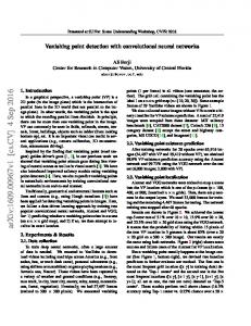
Figure 1. Given a set of lines extracted in calibrated images (left), our goal is to cluster these lines with respect to their (unknownbut-sought) orthogonal vanishing points (right). Each color corresponds to a set of parallel lines.

to which unknown-but-sought VP) and (2) estimate these associated orthogonal VPs, as depicted in Fig 1. This problem has to be differentiated with 2 other situations: calibrated/uncalibrated and pixels/lines. The uncalibrated case, studied in [5][6][15][28], is essentially developed for calibration purpose. The calibrated case (studied in our paper) has been addressed by [2][3], among many others, and these methods will be reviewed in the remaining of this paper. Some approaches also worked on the raw pixels rather than on the extracted lines, like [8][19]. The targeted task is a typical chicken-and-egg problem: if the line clustering is known, then the VPs can be computed and reciprocally, if the VPs are known, the line clustering can be retrieved. Many methods have been proposed since the last 30 years [3], but none of them is fully satisfactory because of the inherent difficulties of the problem. For example, they might get stuck in local minima, the VP orthogonality is complicated to impose and data might contain outliers that must be detected. Thus the line clustering/VP estimation problem still remains an open issue. In contrast to existing works, we present a novel mathematical setup that explicitly maximizes the number of clustered lines in a guaranteed globally optimal manner, while inherently enforcing the orthogonality of the VPs. Specifi-

1. Introduction Parallel lines of the world are projected into perspective images as intersecting lines and their point of intersection is called a vanishing point (VP). Each set of parallel lines is thus associated to a VP. Popular applications of VPs in computer vision are calibration [5][6][28], rotation estimation [2][15][8] and 3D reconstruction [23][7]. Urban environments generally exhibit numerous lines that are either parallel or orthogonal to the gravity direction, which leads to orthogonal VPs (the so-called Manhattan world [8][6][15]). This paper is dedicated to the fundamental problem of line clustering and orthogonal VP estimation. Given a set of lines extracted from a calibrated image, the goal is to (1) determine the line clustering (i.e. find which line belongs 1

cally, we formulate our goal as a consensus set maximization problem over the rotation search space, and solve it efficiently by combining Interval Analysis theory with a branch-and-bound procedure. This paper is organized as follows. First, we recall the concept of equivalent sphere and review existing works. Second, we define the mathematical formulation of the problem. Third, we introduce the concept of interval analysis and present our global optimization method. Finally, we present some experimental results on synthesized data and real images.

2. Sphere Representation and Related Works Most of existing methods perform on a spherical representation of the lines. That is why this section recalls the sphere representation, and then, reviews related works.

2.1. Equivalent Sphere The Gaussian sphere is a convenient way to represent an image when the camera calibration parameters are known. It has been used since [3] for traditional pinhole images and has been extended to the concept of equivalent sphere to handle various types of cameras such as fisheye, omnidirectional, catadioptric and so on [31]. A world line Li is projected onto the sphere as a great circle which is represented by a unit normal vector ni . The great circles of world parallel lines intersect in two antipodal points [4]. They correspond to the vanishing point and are computed by v = ni × nj where ni and nj are the normal vectors of two world parallel lines.

2.2. Existing methods for line clustering Given a set of lines, many methods have been proposed for clustering parallel lines and computing their associated VPs. The common goal is to search for the VPs containing the highest number of lines. Existing methods can be categorized into four main categories. The first category relies on the Hough transform (HT) [3][24][17] to detect the VPs. For each of the possible line pairs, the direction of the intersection of the pair is computed and accumulated in the angular bins. The dominant VP is obtained by selecting the bin that contains the highest number of entries. However, this approach is sensitive to the quantization level of the angular bins and might lead to multiple detections, as confirmed by [26]. In addition, it does not directly impose the orthogonality constraint on VPs since they are detected independently. The second category is based on RANSAC: a simpleyet-powerful method to distinguish the inliers/outliers under an unknown model and compute this model [9]. [1][30][27] applied this approach for line clustering and VP detection. The process starts by randomly selecting two

lines to create a VP hypothesis and then counts the number of lines passing by this hypothesized VP. After a certain number of iterations, it returns the VP (and the associated line clustering) maximizing the number of line inliers. To detect multiple VPs, RANSAC can be sequentially applied on the remaining outliers [27]. The case of “simultaneous” estimation of multiple VPs could be handled by multi-RANSAC [32], an extension of RANSAC to multiple models, or the recent J-linkage algorithm [29] applied by [28]. Whereas interesting results can be obtained by all these methods, an important theoretical limitation of RANSAC and its variants (multi-RANSAC, J-linkage, etc...) is that they do not guarantee the optimality of their solution (in terms of maximizing the number of inliers). Moreover they are non-deterministic: different runs on the same data might produce different results. [16] proposed a method to overcome these limitations, but is limited to linear problems with linear distance functions. Very recently, [20] presented a polynomial approach to impose the VP orthogonality. However this can only consider algebraic cost. In contrast, our approach can deal with (non-linear) geometric cost, which is considered more meaningful [13], and explicitly maximizes the consensus set. The third category refers to a (quasi-)exhaustive search on some of the unknown entities. For example, [4] performs a sampling of the rotation search space to determine the most consistent rotation, i.e. the one which maximizes the number of clustered lines. This method performs quite well in practice and imposes the VP orthogonality. However it depends on the sampling step and the initialization. Furthermore, it does not guarantee to find the best solution even with a very fine sampling. The fourth category directly faces the chicken-and-egg problem, generally following the EM approach [2][8]. It alternates between an expectation (E) step, which estimates the line clustering given the current or hypothesized VPs, and a maximization (M) step, which computes the VPs given the data clustering estimated at the E step. This procedure iterates with the newly computed VPs until convergence. However these methods heavily rely on the initialization and can converge to a local solution.

3. Problem Statement This section states the mathematical formulation of the problem. First, we express it as a consensus set maximization. Secondly, we show that the optimization can be performed on the rotation space instead of directly the VPs.

3.1. Mathematical Formulation As explained in the introduction, line clustering and VP estimation constitute a chicken-and-egg problem. A solution would be to test all the possible (finite but generally untractable) line clustering possibilities and select the one

that maximizes a certain consistency measure. This approach is the most popular. On the contrary, we privilege the other solution: test the VPs (or rotation) and pick up the one that maximizes the VP consistency. It may sound counter-intuitive because the search space of VPs (or rotation) is continuous. But we will show that it actually provides a simpler formulation and can guarantee the VP orthogonality. We adopt the approach of consensus set maximization where the goal is to maximize the number of clustered lines. Let ni be the ith extracted line with i = 1 . . . N . Let the set {v} represents the M orthogonal VPs {v} = {v1 , . . . , vM } where 1 ≤ M ≤ 3. Let the set S of input data be partitioned into an inlier-set Sin ⊆ S and an outlier-set Sout ⊆ S with Sout = S − Sin . To distinguish inliers/outliers, we follow the popular “residual tolerance method” [9]. Concretely, we consider that the line-VP pair (ni , vj ) is an inlier if their geometric (geodesic) distance is lower than a residual tolerance τ , i.e. | arccos(ni · vj ) − π2 | < τ . This τ can be set easily (e.g. 1◦ ) and it is what most of inlier/outlier detection methods do. This inlier pair is noted (ni , vj ) ∈ Sin and ni is clustered to vj . The outlier-set Sout contains the lines that do not belong to any VPs. We allow a line to (accidentally) belong to more than one VP. If needed, a “one-matching” constraint could be applied (cf section 4.3). The problem can be now formulated as a consensus set maximization: max {v}

card(Sin )

(1)

s.t.

| arccos(ni · vj ) − π2 | < τ, ∀(i, j) ∈ Sin ⊆ S (2)

and

kvj k = 1, ∀j and vjT vk = 0, ∀j, k with j 6= k (3)

This formulation says that, given a residual tolerance τ on the geometric geodesic distance, the goal is to find the largest consensus set (i.e. maximize the number of inliers) under an unknown model (here a set {v} of orthonormal VPs), and estimate these VPs. Solving system (1) provides not only the orthonormal VPs maximizing the number of clustered lines but also the clustering information.

3.2. Rotation instead of VPs First of all, working directly on the VPs in system (1) complicates the optimization drastically because the M VPs are encoded by 3M real values, M constraints for their unit length and C2M orthogonality constraints (i.e. the number of combinations of 2 elements out of M ). Moreover the system contains quadratic constraints (orthogonality and unit length) and non-linearities (arccos for the geometric distance). Therefore system (1) is very difficult to solve. As a solution, it is interesting to note that orthonormal VPs can be represented by a single rotation R [4]. Let C be an initial orthonormal basis (e1 , e2 , e3 ), where ej represents the j th axis of the canonical basis, i.e. e1 = (1, 0, 0),

e2 = (0, 1, 0) and e3 = (0, 0, 1). By applying a rotation R to C, a new orthonormal basis is obtained and can represent the orthogonal VPs. Therefore, searching M orthonormal VPs is similar to search one particular rotation. Searching over the rotation space simplifies imposing (1) the VP orthogonality constraints since the initial basis is orthogonal and (2) the VP unit norm constraint since the canonical axes have a unit norm and the rotation is isometric. For now, we write the rotation by R ∈ SO(3), independently of its parametrization, to indicate that it belongs to the set of the three-dimensional rotation group. Therefore the system (1) can be rewritten as: arg max

R∈SO(3)

3 X N X

δ(ni , Rej )

(4)

j=1 i=1

with the inlier function based on the geometric cost: δ(u, v) =



1 0

if | arccos(u · v) − π2 | < τ otherwise

(5)

3.3. Remaining mathematical challenges Despite the reformulation, system (4) still involves some important mathematical challenges. First of all, it constitutes a difficult (chicken-and-egg) non-convex problem. Secondly, the rotation group SO(3) is a complicated space to work on. For example, whereas several rotation parameterizations exist, rotation is not a linear operator with respect to the variables representing its three degrees of freedom (DOF): Euler angles involve non-linear trigonometric functions, quaternions are applied by a quadratic operation and necessitate a bilinear unit-length constraint, axis-angles are converted to another representation, etc... Since the maximization of eq (4) is performed over the rotation, the optimal solution could be found if the cost was examined for every rotation of SO(3). This is impossible in practice because there are infinitely many rotations. An alternative could be an algorithm like Levenberg-Marquardt [18], but it might converge to a local minimum depending on the initialization because of the non-convexity of the function.

4. Proposed Optimization Method This section presents our proposed optimization method to solve the consensus set maximization system (4). Our method combines interval analysis theory and branch-andbound procedure. By an appropriate feasibility test, it successively removes the infeasible rotation intervals and refines the potential intervals. In this section, we first introduce branch-and-bound, then we show how to develop a feasibility test by the help of interval analysis; and finally, we introduce our general optimization framework.

4.1. Introduction to Branch-and-bound For some types of functions, the branch-and-bound algorithm (BnB) can overcome the limitations listed in section 3.3 and provide a globally optimal solution. It has been recently popularized in the computer vision community by [12] (due to space limitation, readers are invited to refer to this paper for detailed information). The basic idea of BnB is to divide the search space into smaller spaces and remove the spaces that cannot contain a solution better than the current one. This removing decision is made by a feasibility test and the associated bounds. BnB has been recently applied to diverse tasks like motion estimation for non-overlapping multi-camera rigs [14] or tilt-pan camera calibration [25]. In order to apply BnB for our problem, we need to parameterize the search space and obtain the lower and upper bounds of the cost function. It will lead us to the development of the first line clustering algorithm whose global optimality is guaranteed.

4.2. Introduction to Interval Analysis The difficulty of BnB is to develop a feasibility test. Concretely, the feasibility test aims at computing the lowest and highest values of the objective function, called bounds, that can be obtained in a studied region of the search space. For example [12][25] manually derived the extreme bounds, but this is applicable only for some “well-arranged” functions. On the contrary, in our application, computing the bounds of a given rotation search space region is challenging, for example because of the non-linearities of the geometric cost and of the rotation operator and the binary output inlier function. Therefore an adapted technique must be developed. To automatically obtain the bounds of a rotation interval, we adopt the theory of interval analysis (IA). Interval analysis [21, 11, 22] is a form of mathematical computation defined on intervals, rather than on real numbers. At the beginning it was mainly employed for bounding the measurement errors of physical quantities for which no statistical distribution was known. A more recent application of IA is to compute provably correct upper and lower bounds on the range of a function over an interval. This property is very interesting because it allows us to know the minimum and the maximum number of possible clustered lines for a given rotation interval. An interval X = [a, b] is defined as [a, b] = {x ∈ R|a ≤ x ≤ b}. A point-interval is an interval where the bounds are equal, i.e. a = b. Interval arithmetic defines a set of operations on intervals. The four elementary interval arithmetic are defined as: • [a, b] + [c, d] = [a + c, b + d] • [a, b] − [c, d] = [a − d, b − c] • [a, b]×[c, d] = [min(ac, ad, bc, bd), max(ac, ad, bc, bd)] • [a, b]/[c, d] = [min( ac , ad , bc , db ), max( ac , ad , bc , db )]

These four interval arithmetic operations are enclosures of point arithmetic operations. Let I be the set of all the intervals. An interval function F : In → In is called an inclusion function for a function f : Rn → Rn if f (X) ⊆ F (X), ∀X ∈ In , where f (X) = {f (x)|x ∈ X} = [inf f, sup f ] over the interval X. By replacing the real arithmetic operators in a real function f by the interval correspondents, we obtain a natural inclusion function FN I ; the range of values of f (x) for x ∈ X is bounded by FN I (X) ≤ f (x) ≤ FN I (X) if there is not the case of a division by an interval containing zero in the evaluation of FN I . In the BnB algorithm, the size of the domain is reduced step by step and so are the lower/upper bounds of the natural extension of the cost function in eq (4).

4.3. Proposed BnB-IA Algorithm We parameterized rotation by Euler angles. If needed, other representations like angle-axis or quaternion can also be used. Let define a rotation angle interval (RAI) as a set of 3 intervals for the roll α, pitch β and yaw γ angles (for general 3D rotation): I = {[α, α], [β, β], [γ, γ]}. For 1D rotation, the RAI would contain only 1 interval, e.g. I = {[α, α]}. Given a RAI I, Algorithm1 computes the associated interval rotation RI and interval VPs v I and returns the lower and upper-bounds of the cardinality Z I = [Z I , Z I ] of the clustered lines (i.e. the minimum and maximum number of possible clustered lines for that interval), by the help of Interval Analysis (cf section 4.2). By abuse of notation, we consider a RAI I as a point-RAI if its bounds Z I is a point-interval, i.e. Z I = Z I . The optional constraint that a line can belong to at most 1 VP (cf P Section 3) can be simply applied by truncating the value j zij to 1 ∀i = 1 . . . N . Our BnB-IA optimization procedure can now be formulated. Analyzing the RAIs is similar to search in a graph. The two most popular search methods are breadthfirst search (BFS, cf Alg2) and depth-first search (DPS). Our BFS algorithm starts with an initial RAI I0 and returns the globally optimal rotation, the associated VPs and line clustering. I0 can be initialized by any algorithms and its volume only influences the convergence speed slightly. The main idea consists in splitting the rotation search space into intervals and analyzing these intervals. Let LI = {I1 , . . . , IN } the list of rotation angle intervals. For each non-point RAI Ik in LI , we subdivide Ik , along the longest angle dimension, into 2 smaller RAIs and compute the lower and upper cardinality bounds Z Ik = [Z Ik , Z Ik ]. The point-RAIs are not studied because their cardinality is a known and fixed integer (point-cardinality). Let Z ∗ be the highest cardinality lower-bound in the cardinality list LZ . Then we remove all the RAIs of LI whose cardinality upper-bound is lower than Z ∗ because it is certain they cannot contain the optimal solution, as illustrated in Fig 2-

Algorithm 1 Lower and upper-bounds by IA Input: an interval of rotation angles I = {[α, α], [β, β], [γ, γ]} Compute the rotation matrix of interval I: RI Compute the 3 VPs vjI by RI with j = 1, 2, 3 for each vj do for each ni do cij = | arccos(ni · vjI ) − π/2| = [cij , cij ] if cij < T then zij = [1, 1] (in any case it is an inlier) else if cij ≥ T then zij = [0, 0] (in any case it is an outlier) else zij = [0, 1] (clustering still unknown) end if end if end for end for P P Return: the clustering bounds Z I = i j zij = [Z I , Z I ]

left. Indeed it means there is at least one interval (the one associated to Z ∗ ) which provides, in the worst case, more clustered lines than these infeasible RAIs. We propose to combine this approach with an additional removal step. Given a RAI I = {[α, α], [β, β], [γ, γ]}, we ˜ γ˜ ) by calculating the avcompute the angle centers (˜ α, β, erage of each angle (e.g. α ˜ = (α + α)/2) and then build the associated rotation. Given this rotation, the clustering can be found by directly testing the constraint of eq (5) and we obtain a potential number ZcI of clustered lines for this interval. The subscript c refers to the fact that the rotation center is tested. This number ZcI provides a key information to remove extra intervals and is inserted in the BnB procedure of Algorithm 2. Figure 3 illustrates the fact that this rotation center test can remove some intervals that cannot be discarded by the lower/upper bound approach. The procedure is repeated, and at each iteration, the size of the remaining RAIs is reduced. Traditional BnB algorithms finish either when the resolution of all the boxes becomes very small (e.g. the difference between the lower and upper angles is less than 0.01◦), or when the cost reaches a certain threshold (which guarantees the result only up to a certain level of accuracy) or when a single candidate remains in the list. These stopping criteria are correct but we propose two alternative criterions for our application. We suggest that the algorithm finishes when (case 1) at least one cardinality point-interval with the maximum upper-bound is obtained or (case 2) at least one interval whose rotation center leads to the maximum upper-bound is obtained.

Figure 2. Management of the interval list. Left: removing the intervals I3 and I5 because their upper-bounds are lower than the maximum lower-bound of the list, ie. Z I1 = 15. Right: the algorithm finishes because the upper-bound of the point-interval I2 equals the maximum upper-bound of the list.

Algorithm 2 BnB and IA line clustering Input: Search space of the rotation angles I0 = {[α, α], [β, β], [γ, γ]} LI = {I0 } (i.e.initialization of the list of rotation angles intervals) repeat for each Ik non-point-interval of LI do Subdivision along the longest dimension and store in LI Compute lower Z Ik and upper Z Ik bounds of the 2 children by Alg.1 and store in LZ Take the rotation center of each child and compute the clustering value ZcIk , and store in LZc end for Z ∗ = maxk {Z Ik ∈ LZ }, Zc′ = maxk {ZcIk ∈ LZc } Remove all Ik from LI such that Z Ik < Z ∗ or Z Ik < Zc′ until ∃l such that Z Il = Z Il = maxk Z Ik (i.e. there exists at least one point interval whose upper-bound is the max upper-bound) or ∃l such that ZcIl = maxk Z Ik (i.e. there exists at least one interval whose rotation center leads to the max upper-bound) Return: I l (i.e. the interval of the rotation angles providing the highest number of clustered lines)

The second case is obvious and the first one is also valid. Because the cardinality intervals of any RAI I has integer bounds, the rotations inside this interval lead to the maximum number of possible clustered lines (cf Fig 2-right). These alternative criterions still guarantee the global optimality of the solution and provide two main advantages. First, all the intervals in the list LI do not have to be studied/subdivided/removed since the algorithm stops when at least one interval is guaranteed to provide the optimal solution. Second, it does not require any heuristic thresholds on the interval resolution or on the cost. Given that the search region contains the solution, our

and searched for M = 3 VPs. The cases where only 1 or 2 VPs exist do not create any difficulties: the extra VPs are simply not associated to any lines.

5.1. Synthesized Data

Figure 3. Removing intervals by testing the rotation center. Left: the traditional lower/upper bound method does not permit to remove any intervals. Right: testing the rotation center (depicted in red for I3 ) permits to remove several intervals (I1 , I2 and I4 indicated in blue).

approach is mathematically guaranteed to converge to the globally optimal solution because BnB is a globally optimal framework when the bounds estimated for each box envelop the values obtained by each element in the boxes [12][25]. In this paper, the bounds are automatically computed by the provably reliable IA technique.

5. Experimental Results This section presents experimental results for both synthesized and real data. Additional results for omnidirectional videos composed of hundreds of images from the Google Street View dataset are available on the authors’ website. We developed our method in Matlab and implemented first order inclusion for IA. If necessary, higherorder inclusion functions could also be used [22]. For comparison purpose, we also implemented several existing works reviewed in section 2.2: • Hough transform [24] with different number of bins (100, 200 and 300 for each angle on the sphere surface) • RANSAC with a sequential search of the VPs (referred to as “Seq-Ransac”) [27] • RANSAC with a simultaneous search of the VPs (referred to as “Sim-Ransac”): 3 lines are randomly selected, intersection of the first two gives v1 and intersection of the third line and the plane orthogonal to v1 gives v2 . Finally, the cross-product of v1 and v2 provides v3 • EM algorithm [2] initialized by HT • the quasi-exhaustive search of [4] (referred to as “Exhaus”) with various sampling rates: 0.2◦ (for very fine sampling), 0.5◦ (intermediate) and 1◦ (coarse) with an offset of ±10◦ If a method does not provide orthogonal VPs, we applied a popular orthonormalization based on the Frobenius norm to find the “nearest” orthogonal solution [10] and then recounted the inliers. In all the experiments, we set τ = 1◦

In this section, we intend to check how well our BnBIA algorithm works, especially in terms of optimality and convergence. For this aim, we synthesized data containing 2 or 3 orthogonal clusters of 5 to 100 parallel lines. To mimic real situations, the orientations of the line normals have been corrupted by a gaussian noise of 3◦ and some outlier lines have been added. Given the line normals, the goal is to cluster the lines and estimate their associated VPs. Figure 4 illustrates a representative comparison of the number of inliers found by the proposed method and several existing works. Since RANSAC-based methods are not deterministic, we run them 1000 times and display their distribution with a boxplot. As expected, Sim-Ransac performs better than Seq-Ransac in average because it inherently imposes the VP orthogonality. The quasi-exhaustive search works quite well (when the nb of samples is tractable) and EM manages to improve the results of Hough-100. Our method obtains 32 inliers, which exactly corresponds to the number of synthesized inliers. On the contrary, the existing works span between 20 and 30 inliers. In all the experiments, our number of inliers was always higher or equal than the one obtained by the existing works. Apart the mathematically guaranteed global optimality of our algorithm, some reasons exist to explain why the existing works do not perform as well. First, HT and the quasiexhaustive search might miss the global solution because of the search space sampling/quantization. A second reason is that RANSAC methods can only hypothesize VP models from the selected lines, i.e. cannot generate VPs not directly supported by the randomly selected lines.

Figure 4. Comparison of the number of inliers detected by the proposed approach and some existing works (cf text for more details).

To illustrate the convergence of the algorithm, two kinds of figures are of main interest: the upper- and lower-bound evolution curve and the shrink of the total volume of the remaining RAIs. To measure its speed, we used the number of iterations, rather than the absolute CPU time because it depends on the language and the implementation quality. Figure 5 illustrates the convergence of the global lower and upper bounds for a representative experiment with 2 VPs, 50 lines per VP and 20% of outliers. It takes only 318 iterations (about 3 seconds) to find that the maximum cardinality is 100 lines. The total volume of the parameter space drops very quickly. It is interesting to note that the volume does not have to reduce to 0 since our algorithm stops as soon as there is at least one point interval whose upper-bound equals the maximum upper-bound, as explained in section 4.3. We also analyzed the effects of the BnB search region size (from ±10◦ to ±40◦ for each angle), data amount (from 1 to 3 VPs and from 0 to 100 lines per VP), noise level (from 0◦ to 5◦ ) and proportion of outliers (from 0% to 80%). First of all, it is important to emphasize that extensive experiments showed that neither the search region size, nor the nb of VP/lines nor the level of added noise nor the fraction of outliers affected the BnB-IA algorithm’s convergence, i.e. the lower and upper-bounds always converged. Second, we also always obtained a higher or equal number of inliers compared to existing works. Third, the algorithm generally runs in a couple of seconds, which is fast compared to previous works related to BnB [12]. RANSAC and HT-based methods are obviously faster but, as discussed previously, they lack in exactness and cannot guarantee the optimality of their solution. Experiments also demonstrated the scalability of the method. For example, Figure 6 illustrates that a much larger search region (from ±10◦ to ±40◦ that is to say 43 = 64 times larger) affects the number of BnB iterations very slightly and, in turn, the execution time. Moreover, since each box of the BnB can be analyzed independently, our method can be implemented on GPUs to run in parallel, which greatly reduces the execution time.

5.2. York urban database for real images In order to verify the clustering obtained by our algorithm on real images, we tested it on the York urban

bounds value

Lower bound Upper bound

150 100 50 0 0

100

200

300

iteration index

400

remaining volume in %

100

200

90 80 70 60 50 40

50

100 150 200 iteration index

250

300

Figure 5. Convergence of the upper and lower cardinality bounds (left) and convergence of the volume of the search space (right)

Figure 6. Distribution of the number of BnB iterations of our algorithm, for 1000 runs, with respect to the search region size: ±10◦ and ±40◦ around the synthesized rotation on the same random data composed of 2 VPs, 10 lines per VP and 20% of outliers.

Figure 7. Typical results obtained by our method on the York urban database [8] for outdoor with 2 VPs (top) and indoor with 3 VPs (bottom). Left: set of extracted lines provided in the database. Right: automatic line clustering by our method.

database [8] which contains the true clustering obtained manually. This database consists of 102 perspective indoor and outdoor images of man-made environments with their associated intrinsic calibration parameters. Each image in the database contains 2 or 3 VPs, a set of line segments manually extracted (119 lines in average without outliers) and their ground truth clustering. To reduce input data noise, we filtered out the segments whose length is less than 5% of the image height. Given the set of line segments, we apply our algorithm to find the clustering and then compare it with the ground truth. For each line clustered by our algorithm, we successfully obtain the true clustering, which demonstrates the correctness of our approach. Figure 7 shows some representative results obtained by our method.

6. Conclusion Given a set of lines extracted in calibrated images, this paper faced the problem of line clustering and orthogonal

VP estimation in urban environments. Existing works have several important limitations (sphere quantization, search space sampling, initialization, randomness of the results, post-orthonormalization, etc...), the most important one being that they all might lead to a local minimum. In contrast, our first contribution is an algorithm that solves the problem in a mathematically guaranteed globally optimal manner: we can find the line clustering and the associated VPs leading to the globally optimal largest number of clustered lines. The optimization is performed by a branch-and-bound framework coupled to the Interval Analysis theory. Our second contribution is the inherent enforcement of the VP orthogonality. Moreover, the proposed approach can handle the case of any number of orthogonal VPs (i.e. 1, 2 and 3), be applied for a large range of images (e.g perspective and omnidirectional) and efficiently deals with outliers. Our algorithm has been validated successfully on both synthesized data and challenging real images.

7. Acknowledgments This work was partly supported by the National Research Foundation of Korea Grant funded by the Korean Government (NRF-2011-371-G00004 and MEST No.20110018250) and by Predict program from the Japanese government. This research, which has been partially carried out at BeingThere Centre, is also supported by the Singapore National Research Foundation under its International Research Centre @ Singapore Funding Initiative and administered by the IDM Programme Office.

References [1] D. G. Aguilera, J. G. Lahoz, and J. F. Codes. A new method for vanishing points detection in 3D reconstruction from a single view. In Proceedings of ISPRS comission, 2005. 2 [2] M. E. Antone and S. J. Teller. Automatic recovery of relative camera rotations for urban scenes. In CVPR’00. 1, 2, 6 [3] S. T. Barnard. Interpreting perspective image. Artificial Intelligence Journal, 1983. 1, 2 [4] J.-C. Bazin, C. Demonceaux, P. Vasseur, and I. Kweon. Rotation estimation and vanishing point extraction by omnidirectional vision in urban environment. The International Journal of Robotics Research, 2012. 2, 3, 6 [5] B. Caprile and V. Torre. Using vanishing points for camera calibration. IJCV’90. 1 [6] R. Cipolla, T. Drummond, and D. Robertson. Camera calibration from vanishing points in images of architectural scenes. In BMVC’99. 1 [7] A. Criminisi, I. Reid, and A. Zisserman. Single view metrology. IJCV’00. 1 [8] P. Denis, J. H. Elder, and F. J. Estrada. Efficient edge-based methods for estimating manhattan frames in urban imagery. In ECCV’08. 1, 2, 7 [9] M. A. Fischler and R. C. Bolles. Random sample consensus: A paradigm for model fitting with applications to image

[10] [11] [12] [13]

[14]

[15] [16] [17]

[18]

[19]

[20] [21] [22] [23] [24] [25]

[26] [27]

[28] [29] [30] [31]

[32]

analysis and automated cartography. In Comm. of the ACM, 1981. 2, 3 G. Golub and C. V. Loan. Matrix Computation. Johns Hopkins University Press, Maryland, third edition, 1996. 6 E. Hansen. Global Optimization Using Interval Analysis. 1992. 4 R. Hartley and F. Kahl. Global optimization through rotation space search. IJCV’09. 4, 6, 7 R. I. Hartley and A. Zisserman. Multiple View Geometry in Computer Vision. Cambridge University Press, second edition, 2004. 2 J. H. Kim, H. Li, and R. Hartley. Motion estimation for nonoverlapping multi-camera rigs: Linear algebraic and L∞ geometric solutions. PAMI’09. 4 J. Kosecka and W. Zhang. Video compass. In ECCV’02. 1 H. Li. Consensus set maximization with guaranteed global optimality for robust geometry estimation. In ICCV’09. 2 M. J. Magee and J. K. Aggarwal. Determining vanishing points from perspective images. Proc Computer Vision, Graphics and Image Processing, 1984. 2 D. Marquardt. An algorithm for least squares estimation of nonlinear parameters. SIAM Journal of Applied Mathematics, 1963. 3 A. Martins, P. Aguiar, and M. Figueiredo. Orientation in Manhattan: Equiprojective classes and sequential estimation. PAMI’05. 1 F. M. Mirzaei and S. I. Roumeliotis. Optimal estimation of vanishing points in a manhattan world. In ICCV’11. 2 R. Moor. Interval Analysis. 1966. 4 R. Moor, R. B. Kearfott, and M. Cloud. Introduction to Interval Analysis. 2009. 4, 6 P. Parodi and G. Piccioli. 3D shape reconstruction by using vanishing points. PAMI’96. 1 L. Quan and R. Mohr. Determining perspective structures using hierarchical hough transform. PRL’89. 2, 6 Y. Seo, Y. Choi, and S. Lee. A branch-and-bound algorithm for globally optimal calibration of a camera-and-rotationsensor system. In ICCV’09. 4, 6 J. A. Shufelt. Performance evaluation and analysis of vanishing point detection techniques. PAMI’99. 2 S. Sinha, D. Steedly, R. Szeliski, M. Agrawala, and M. Pollefeys. Interactive 3D architectural modeling from unordered photo collections. In SIGGRAPH Asia’08. 2, 6 J. P. Tardif. Non-iterative approach for fast and accurate vanishing point detection. In ICCV’09. 1, 2 R. Toldo and A. Fusiello. Robust multiple structures estimation with J-linkage. In ECCV’08. 2 H. Wildenauer and M. Vincze. Vanishing point detection in complex man-made worlds. In ICIAP’07. 2 X. Ying and Z. Hu. Can we consider central catadioptric cameras and fisheye cameras within a unified imaging model. In ECCV’04. 2 M. Zuliani, C. S. Kenney, and B. S. Manjunath. The multiRANSAC algorithm and its application to detect planar homographies. In ICIP’05. 2