Efficient Grasping from RGBD Images: Learning using a new. Rectangle ... This rectangle, which we call a 'grasping rectan- gle', actually .... The center of the.
Efficient Grasping from RGBD Images: Learning using a new Rectangle Representation Yun Jiang, Stephen Moseson, and Ashutosh Saxena Abstract— Given an image and an aligned depth map of an object, our goal is to estimate the full 7-dimensional gripper configuration—its 3D location, 3D orientation and the gripper opening width. Recently, learning algorithms have been successfully applied to grasp novel objects—ones not seen by the robot before. While these approaches use low-dimensional representations such as a ‘grasping point’ or a ‘pair of points’ that are perhaps easier to learn, they only partly represent the gripper configuration and hence are sub-optimal. We propose to learn a new ‘grasping rectangle’ representation: an oriented rectangle in the image plane. It takes into account the location, the orientation as well as the gripper opening width. However, inference with such a representation is computationally expensive. In this work, we present a two step process in which the first step prunes the search space efficiently using certain features that are fast to compute. For the remaining few cases, the second step uses advanced features to accurately select a good grasp. In our extensive experiments, we show that our robot successfully uses our algorithm to pick up a variety of novel objects.
I. I NTRODUCTION In this paper, we consider the task of grasping novel objects, given its image and aligned depth map. Our goal is to estimate the gripper configuration (i.e., the 3D location, 3D orientation and gripper opening width) at the final location when the robot is about to close the gripper. Recently, several learning algorithms [1–3] have shown promise in handling incomplete and noisy data, variations in the environment, as well as grasping novel objects. It is not clear, however, what the output of such learning algorithms should be—in this paper we discuss this issue, propose a new representation for grasping, and present a fast and efficient learning algorithm to learn this representation. In a learning setting for grasping, the problem is formulated as: given image/range data, predict a ‘representation’ of the gripper configuration. Typically, this representation is a low-dimensional projection of the full gripper configuration (which is up to 7-dimensional for a two-fingered gripper) at the final grasping stage. Several representations have been proposed: Saxena et al. [1] proposed to use a 2D ‘grasping point’ for this representation. Le et al. [3] used a pair of points as their representation. These representations suffer from the problem that they are not a faithful representation of the 7-dimensional configuration, so learning is used to predict a part of the configuration while other dimensions are left to be estimated separately. Yun Jiang, Stephen Moseson and Ashutosh Saxena are with the Department of Computer Science, Cornell University, Ithaca, NY.
{yunjiang,scm42,asaxena}@cs.cornell.edu
Fig. 1: Given the image (left) and depth map (right), our goal is to find the oriented rectangle (shown with red and blue edges). The rectangle indicates not only where to grasp the shoe and the gripper’s orientation, but also the gripper’s opening width and its physical size (shown by the length of the red and blue lines respectively). Being able to pick up such an object would be useful for object-fetching robots, such as [4].
Our new representation of the 7-dimensional grasping configuration (that takes into account the location, orientation and gripper opening width) is an oriented rectangle (Fig. 1) from which the 7-dimensional gripper configuration can be obtained. This rectangle, which we call a ‘grasping rectangle’, actually represents a ‘set’ of grasping configurations. We describe this representation and its benefits in Section III. However, finding the best grasp with this representation is computationally expensive because the number of possible rectangles is quite large. We therefore present a two-step learning algorithm to efficiently learn this representation. First, we describe a certain class of features that makes the inference in the learning algorithm fast. Second, we describe certain advanced features that are significantly more accurate but take more time to compute. Each step is learned using the SVM ranking algorithm [5]. With the top results from the first step, we then run a second classifier in a cascade that is more accurate (but slower) in order to find the top choice. Using the point cloud, we convert this representation to the full 7dimensional gripper configuration and execute the grasp. Our results show that our representation is a better encoding for grasping configurations as compared to the previous ‘grasping point’ representation. In extensive experiments using an industrial arm (that lacks any kind of haptic or force feedback), our method successfully picks up a wide variety of objects (window wipers, wire strippers, shoes, etc.) even from categories not seen by the robot before. II. R ELATED W ORK Most previous work in robotic grasping requires full knowledge of 2D or 3D models of objects. Based on this precise information, methods such as ones based on forceclosure [6,7] and form-closure [8] focus on designing control
and planning algorithms to achieve successful and stable grasps. We refer the reader to [9–11] for a more general survey of past work in robotic grasping. In real-world grasping, the full 3D shape of the object is hard to perceive. Some early work considers only objects of simple shapes to address this problem. For example, Miller et al. [12] used heuristic rules to generate and evaluate grasps for three-fingered hands by assuming that the objects are made of basic shapes such as spheres, boxes, cones and cylinders, each with pre-computed grasp primitives. Other methods focus on grasping 2D planar objects using edges and contours to determine form and force closure. Piater [13] estimated 2D hand orientation using K-means clustering for simple objects (specifically: squares, triangles and round “blocks”). Morales et al. [14] calculated 2D positions of three-fingered grasps from 2D object contours based on feasibility and force-closure criteria. Bowers and Lumia [15] also considered grasping planar objects by classifying them into a few basic shapes, and then used pre-scripted rules based on fuzzy logic to predict the grasp. Pelossof et al. [16] used support vector machines to estimate the quality of a grasp given a number of features based on spin images; however this work was done in simulation and it is not clear how it would apply to real-world grasping. Hsiao et al. [17, 18] used partially observable Markov decision processes to choose optimal control policies for grasps, and also used imitation learning for whole-body grasps. Another notable work is GraspIt [19, 20] where a large database of 3D objects was used to evaluate the grasps. However, all these methods assumed full knowledge of the 3D object model, and their main method of testing was through a simulator. For grasping known objects, one can also use learning-by-demonstration [21]. Klingbeil, Saxena and Ng [22] used supervised learning in order to detect and turn door handles. Using learning algorithms to predict grasps helps in several ways. First, it provides a degree of generalization to grasping, thus making it applicable to previously unseen objects. Second, it is trained on data, making it possible to add more features (as well as data) in order to increase the performance. Saxena et al. [1, 2, 23] showed that a ‘grasping point’ could be estimated from the image using supervised learning algorithms, and that this method generalized to a large number of novel objects. However, their grasping point representation only indicated where to grasp, and other parameters such as gripper orientation were left to be estimated by other methods (e.g., [24]). In later works, Saxena et al. [25] also used point clouds for grasping. Rao et al. [26] used depth information to segment the objects from the background in order to increase the performance in cluttered environments. Le et al. [3] questioned whether a ‘grasping point’ is a good representation to learn, and instead proposed a new representation based on a pair of points. However even this representation suffers from some limitations that we describe in the following section.
Fig. 2: Examples of grasping rectangles. A 2D rectangle can be fully represented by its upper-left corner (rG , cG ), length mG , width nG and its angle from the x-axis, θG . For some objects, like a red lid in the right image, there can be multiple possible grasping rectangles.
III. R EPRESENTATION In our setting, the robot takes an image along with an aligned depth map from a stereo camera. (Other sensors can also obtain such a depth map/disparity image, such as [27] or [28].) The depth map can be used to compute a disparity image or a 3D point cloud and vice versa. The representation used for learning the grasping point should be a sufficient statistic of all seven dimensions—the 3D location, the 3D orientation and the distance between the two fingers. Furthermore, it should also be able to accommodate physical constraints, such as the maximum opening width of the gripper, in the learning algorithm. We define our representation to be an oriented rectangle in the image plane (see Fig. 2). The first and the third edge of the rectangle (shown as blue lines) are where the two jaws of the gripper are to be positioned for grasping. The second and fourth (shown as red lines) depict the gripper opening width and the closing direction. Formally, let I be the n by m image containing the object to be picked up. A 2D rectangle G is uniquely specified by 5 parameters (rG , cG , nG , mG , θG ). rG and cG refer to the upper-left corner of the rectangle (see the green dot in Fig. 2). mG and nG are the dimensions of the rectangle. And θG is the angle between the first edge and x-axis, as shown in the left image in Fig. 2. Notice that rG , cG , nG and mG are with respect to the image after rotating it by θG degrees. Note that our representation has strong parallels with the ‘bounding box’ representation used for object detection in the computer vision community that has decades of work behind it and has been quite successful (e.g., [29]). Now we describe how the rectangle is a full representation of the 7-dimensional gripper configuration. The center of the rectangle is used to obtain the 3D position p from the point cloud. We use the width of the rectangle to compute the gripper opening width. For 3D orientation, θG gives us one angle—rotation in the image plane (about the camera axis). For the other two orientation angles, the configuration of the 3D points in the rectangle could be used. However, given only one view of the object, we found that the normal to the image plane indicates a good direction to approach. Another interpretation, more applicable for robots with ‘thin’ fingers, is that a grasping rectangle actually represents a ‘set’ of grasping configurations rather than just one. For example, for a long object such as a white-board marker, the
ground-truth label for the grasping rectangle would be a long rectangle aligned with the marker and covering almost its full length. Any grasping configuration from this set would be a good grasp. A collection of grasps is more likely to capture the important features and patterns of grasp than an individual pair of points. Compared with some previous work in which one grasping point [1,2] or a pair of points [26] is used to represent grasps, our representation has two advantages: • First, our grasping rectangle explicitly models the physical size of the gripper (i.e., a parallel plate gripper has a certain width), which cannot be captured using only a single point [1], or a pair of points [26]. • Second, a grasping rectangle strictly constrains the boundary of features, i.e., the features are computed only from within the rectangle and the entire rectangle is used. On the other hand, a grasping point or a pair of points have an arbitrary support area (e.g., an area of some radius around the points)—which is not matched to the physical space that the gripper fingers will occupy. While our representation captures the aforementioned properties, it is still only useful for single-view grasping. Determining a grasp using multiple views of the object requires additional thought (beyond the scope of this paper). This also draws strong parallels to the field of multi-view object detection [30] in the computer vision community. While our representation and learning algorithms works for two-jaw grippers, it can potentially represent grasps for multi-fingered hands as well. Multiple fingers could be represented using different locations within the rectangle. This is an interesting direction for future research. IV. A LGORITHM A. Overview Our algorithm takes an image and an aligned depth map as input, which we will refer to as a single image with four values at each pixel—RGBD—where D represents depth. Our goal is to find the optimal grasping rectangle(s) in this image. (As explained in Section IV-C, it is possible to have multiple valid grasping rectangles.) To measure ‘optimal’ quantitatively, we first define a score function which assigns a real number to a rectangle based on its features. Thus our goal becomes finding the rectangle with the highest score in the image. Using an exhaustive search is infeasible in terms of time complexity. However if both the score and features can be computed incrementally, the search space can be significantly reduced. But this requirement excludes some computationally more expensive features that more accurately capture the aspects of a good grasp. In order to balance this trade-off between efficiency and accuracy, we design a two-step process. In the first step we use features that allow incremental computation of the score function and use them to narrow down the search space from tens of millions down to a hundred rectangles. In the second step, we then use more sophisticated features to refine the search and finally get the optimal rectangle. The first step is fast but inaccurate, while the second is accurate but slow.
In the following section we will define our score function, our learning method, and then describe our two-step inference process and the different types of features it uses. B. Score Function For a rectangle G in I, we use φ (G) to denote the features of G. Assume there are k features, i.e., φ (G) ∈ Rk . The score function f (G) should take φ (G) as the input, and our goal is to find the rectangle with highest score: G∗ = arg max f (G) G
(1)
We define our score function to be a linear function of the features, k
f (G) = wT φ (G) = ∑ wi φi (G)
(2)
i=1
Defining f as a linear function of features is quite common in machine learning algorithms such as SVM [31] and linear regression [32]. Besides simplicity, a linear function has another merit in that it accelerates the search process, which we will discuss in Section IV-D. C. Learning the score function Our goal is to enable our robot to grasp novel objects, and therefore we use supervised learning to learn the parameters w from the labeled training data (see Section VII-A). This is motivated by Saxena et al. [1, 2, 33] and Le et al. [3] who show that using learning algorithms provides some level of generalization—with the parameters for a large number of features learned from a large amount of labeled data. This is also more robust as compared to hand-written rules or manually computed parameters for a few features (such as edges) from the images. In our supervised learning approach, similar to [3], we note that there can be more than one good grasp, and among these, some grasps may be more desirable. For example, a screwdriver may be grasped both by the handle or the shaft, however the handle is preferred due to its size, material and such. This makes the boundary between a good and bad grasping rectangle somewhat vague. In this case, ranking different rectangles makes more sense than just classifying them into ‘good’ and ‘bad’ categories. Thus we consider this as a ranking rather than a classification task. Specifically, for each image in the training set, we manually label ranks 1 to 3 for the grasping rectangles and randomly sample some bad ones. We then use SVM-rank [5] to learn the weights, w. D. Inference: Fast Search In order to find the rectangle with highest score (see Eq. 1), one can simply go through all the rectangles and compare their scores. While such a brute-force method may have been fine if we were finding a “grasping point” [1], in the case of rectangles it becomes very expensive. Even if we disregard the orientation of the rectangle for now, this bruteforce search would have to consider four variables rG , cG , nG and mG respectively to specify G, which takes O(n2 m2 ) time, for an image of size n by m. For every G, we would
have to extract features and compute the score in O(k). Thus in total, direct exhaustive search costs at least O(n2 m2 k). We note that finding the highest-score rectangle is actually equivalent to the classic problem of finding the maximumsum submatrix [34], for which several efficient algorithms exist. We realize that if the score of the rectangle can be decomposed as a sum of scores of each pixel then our problem can be solved efficiently. This is because of our linear score function that enables us to decompose the score function as a sum of scores over the individual pixels. Suppose we know f (G) for a rectangle G, and we add ∆G to get G0 = G ∪ ∆G. If our features are such that: φi (G ∪ ∆G) = φi (G) + φi (∆G)
Fig. 3: Spatial histograms. On the left, a grasping rectangle for a martini glass is divided into three horizontal strips: top, middle and bottom. The right figure shows the corresponding histogram of depths for each region. Notice that the histogram for the middle region (green) looks very different compared to that of the two side regions (red and blue).
F2
F1
then we can compute f (G0 ) as:
F3
k
f (G0 ) = f (G ∪ ∆G) = ∑ wi φi (G ∪ ∆G) = f (G) + f (∆G) i=1
As a result, we only need to calculate f (∆G), which costs far less time than computing f (G0 ) all over again. More formally, if all features satisfy, φi (G) =
φi (I(x, y)),
∑
∀i = 1, . . . , k
(3)
(x,y)∈G
where φi (I(x, y)) is the value of feature i at pixel (x, y). Then we can calculate f (G) in the following way: k
f (G) = =
wi φi (G) i=1 k rG +nG cG +mG
∑
∑ ∑ ∑
wi φi (I(x, y))
i=1 x=rG y=cG rG +nG cG +mG k
=
∑ ∑ ∑ wi φi (I(x, y))
x=rG y=cG i=1 rG +nG cG +mG
=
∑ ∑
x=rG
F(x, y)
y=cG
In the last step, we have defined a new matrix F (of the same size as image I), such that F(x, y) represents the score of pixel (x, y), i.e. F(x, y) = ∑ki=1 wi φi (I(x, y)). (The next section describes which features satisfy this property.) Now our goal in Eq. 1 transforms to: given matrix F, find a rectangle (or submatrix) within it with the largest sum. This is exactly the classical problem of finding the maximum-sum submatrix [34]. We use an incremental search algorithm1 to reduce the time complexity from O(n2 m2 k) 1 We first fix the range of rows of the submatrix, i.e. r and n , and G G rG +nG compute the score of each column within this range F 0 (y) = ∑x=r G F(x, y) for y = 1, . . . , m. Starting with the first column, we keep track of the current sum s and the largest sum s∗ (each initialized to zero), as well as their corresponding submatrices. With each additional column, y, we add F 0 (y) to the current sum, s ← s + F 0 (y), and update s∗ and G∗ if necessary. If s is negative we discard the first y columns and resume the search from the (y + 1)th column by setting s back to 0, and G to 0. / This is because if the current sum is negative, then excluding this part is better than including it. More details and proof can be found in [35]. Thus, we are guaranteed to find the highest-score rectangle. After enumerating rG and nG we only need a one-pass scan of each column to find the maximum-sum submatrix.
Grasp Rectangle
0.5 0.7 0.6 0.2 0.2 1.0 1.0 0.2 0.2
0.4 0.5 0.2 0.6 0.5 0.7 0.7 0.6 0.5
0.2 0.2 1.0 0.2 0.4 0.5 0.5 0.2 0.4
0.6 0.5 0.7 1.0 0.2 0.2 0.2 1.0 0.2
0.2 0.4 0.5 0.7 0.6 0.5 0.5 0.7 0.6
1.0 0.2 0.4 0.5 0.2 0.2 0.4 0.5 0.2
Fig. 4: Applying spatial histogram features to fast search. Every pixel has three scores from matrices F1 , F2 and F3 . Which score to use is decided by its place in the rectangle. For example, if a pixel is in the middle part, then its score comes from F2 . The score of a grasping rectangle is the sum of scores of its three sub-rectangles.
down to O(n2 m). We also need to first compute the score of each pixel, i.e. matrix F, in time O(nmk). Therefore the overall time complexity is O(nmk + n2 m), as long as all the features satisfy Eq. 3. E. Grasping Features for Fast Search As Eq. 3 implies, features that are capable of accelerating the search must be computed independently on each pixel. For instance, the sum of grayscale intensity values in the rectangle is a possible feature, while their mean value is not. Similarly, histograms are a good source of such features because calculating a histogram of G equals the sum of the histogram of each pixel in G. In this work, we use 17 filters to capture the information of color, textures and edges [2, 36]. Among them, six oriented edge filters and nine Law’s masks are applied on the intensity channel, and two averaging filters are convolved on the two color channels respectively. Spatial Histogram Features: Although a histogram has the potential to describe the overall distribution in the rectangle, it is not always good at finding patterns at different parts of the rectangle. Specifically, if we divide the grasping rectangle into horizontal strips (e.g., as shown in Fig. 3), each strip tends to have its own unique pattern. For instance, if we try to grasp a martini glass, the middle part of the rectangle should be the stem and the two sides should be the background. This
corresponds to a depth map where the middle strip has closer depths than the sides. As showed in Fig. 3, we evenly divide the rectangle into three horizontal sub-rectangles and compute features for each one separately. Thus the feature space is tripled, and our search algorithm requires a modification. We use w1 , w2 and w3 to represent the weights for the top, middle and bottom sub-rectangles respectively. A rectangle’s score is now the sum of the scores of the three sub-rectangles. Instead of having one matrix F, we now must compute three matrices F1 , F2 and F3 and use these to compute the score of each sub-rectangle separately2 , as shown in Fig. 4. After tripling the feature space the time complexity still remains O(nmk + n2 m). Using 17 filters and 5-bin histograms for each of the three sub-rectangles, we now have 17 × 5 × 3 = 255 total features.
are three values from these histograms. Let φT , φM , φB denote values corresponding to the top, middle and bottom subrectangle respectively. For our advanced features, we add the features φT /φM , φB /φM and φT φB /φM , as well as the mean and median from the depth map to get a total of 522 features.
(a) histogram of positive examples
F. Advanced Features While histogram features are good for fast pruning of the search space, more powerful features are needed for estimating the grasping rectangle accurately. In particular, we must have features that capture the correlations between the three sub-rectangles. For example, one possible relation is that the average depth of both the top and bottom sub-rectangles should be larger than that of the middle one. For illustration, assume the three mean depths of the three sub-rectangles are d1 = d + ∆d, d2 = d and d3 = d + ∆d (think the stem of a martini glass). If only the histogram features are used, the resulting model will have negative w2 and positive w1 and w3 , meaning that rectangles with large d1 and d3 and small d2 are preferred. However, it will also assign a high score to a rectangle with small d10 = d, d20 = d but much larger d30 = d + 2∆d (e.g., a rectangle not lying on the stem of the martini glass), since the score from d3 and d1 are additive. It would be better to use the criterion d1 > d2 and d3 > d2 . However, because the depths are noisy we cannot rely on such hard constraints. We instead use non-linear features, such as dnl = d1 d3 /d22 to represent this preference. To verify that this feature can help distinguish grasping rectangles, we plot the histogram of positive/negative examples in Fig. 5a and 5b respectively. In the left image, values are almost distributed from 0.5 to 1, while in the right image the distribution is centered around 1, and is very symmetric. This coincides with the fact that for a true grasping rectangle d1 d3 /d22 is more likely to be less than 1. Based on the existing 255 features from the histograms, we use more advanced features to improve the model. In each filter, we have three 5-bin histograms for three sub-rectangles (top T , middle M and bottom B), so that for each bin, there 2 They represent the individual pixel’s score when it is in a different part of the rectangle. Recall that F 0 ( j) equals the score of jth column from row rG to rG + nG , and now we must re-define F 0 ( j) as rG +nG /3 rG +2nG /3 rG +nG F1 (i, j) + ∑i=r F2 (i, j) + ∑i=r F3 (i, j). Please re∑i=r G G +nG /3+1 G +2nG /3+1 fer to Fig. 4 for a better understanding of F1 , F2 and F3 . By pre-computing F˜t (i, j) = ∑ii0 =1 Ft (i0 , j), t = 1, 2, 3, then F 0 ( j) = (F˜1 (rG + nG /3, j) − F˜1 (rG − 1, j)) + (F˜2 (rG + 2nG /3, j) − F˜2 (rG + nG /3, j)) + (F˜3 (rG + nG , j) − F˜3 (rG + 2nG /3, j)), whose complexity is O(1).
(b) histogram of negative examples
Fig. 5: Histogram of feature dnl = d1 d3 /d22 . The x axis is the value of dnl and the y axis is the number of positive/negative rectangles.
G. Learning and Inference in Second Step In the second step, the form of the SVM ranking model is the same as that described in Section IV-C. We use the first model for searching the top T -ranked rectangles, and then use the second model to rank those T rectangles. Notice that in the first step, searching for the top T rectangles can be done in O(n2 (m + T )). In the second step ranking, we extract features of those T rectangles and compare their score using the second model. The complexity for computing each feature is as much as O(nm), making the total second step complexity O(nmkT ). Fig. 6 shows an example output from the two-step process. Notice that in the left image, most of the rectangles are located near the head or handle of the brush. After ranking them using more sophisticated features, the top rectangle is found to lie directly over the handle. Finally, for the rectangle’s orientation, we discretize angles in 15◦ intervals. For each orientation, we rotate the image before applying the filters and search. V. ROBOT H ARDWARE We use an Adept Viper s850 arm with six degrees of freedom, equipped with a parallel plate gripper that can open to up to a maximum width of 5cm. The arm weighs 29kg and has a rated payload of 2.5kg, but our gripper can only hold up to 0.5kg. The arm, together with the gripper, has a reach of 105cm. The arm has a repeatability of 0.03mm in
(a) The top 100 rectangles after the first-step search.
(b) The top 3 rectangles after the second-step rank.
Fig. 6: Example results from two-step search.
XYZ positioning, but because our gripper has some play in its gears our estimated repeatability with the gripper becomes 0.1mm. The camera-arm calibration was accurate up to an average of 3mm. The Adept Viper is an industrial arm and has no force or tactile feedback, so even a slight error in positioning can result in a failure to grasp. For perception, we use a Bumblebee2 stereo camera (manufactured by PointGrey) that provides 1024 × 768 resolution stereo images. We obtain the disparity image, depth map and point-cloud using the camera library. VI. E VALUATION M ETRICS IN L EARNING For an actual grasp to succeed, the predictions must satisfy several criteria: 1) The center point of the gripper must be at the correct location. 2) All three orientation angles must be correct. 3) The area where the object is grasped must be wide enough to accommodate the open gripper. Furthermore, these factors are interrelated, i.e., one center point could work for a particular orientation but not others. The metric described in [1] counts a prediction as correct if the predicted “grasping point” is within a certain distance of the ground-truth labeled point. This metric only satisfies the first criteria, and ignores the others. Our ‘rectangle metric’ that we describe below considers all the criterion above, but we also evaluate on Saxena et al.’s old ‘point metric’: ‘Point’ metric: Our prediction is a rectangle. Therefore, we first obtain the center of the rectangle and then if the distance of the center of the rectangle is within a certain threshold from the ground-truth grasping point labels, we treat it as a correct ‘Point’ prediction. We will later show that this metric is not always reliable, and slightly overestimates the performance (when compared to actual robotic experiments)—one of the reasons is that it does not consider orientation. ‘Rectangle’ metric: Let G be the predicted rectangle and G∗ be the ground truth. We first classify all the predictions that have an orientation error of more than 30 degrees as incorrect. For the rest of the predictions we measure the amount of area that G and G∗ overlap in order to estimate how close the prediction is to the ground-truth label. More formally, we define a prediction to be correct if (G∩G∗ )/G ≥ 0.5. Finally, if there are multiple grasping rectangles, we choose the one with the maximum overlap. VII. E XPERIMENTS A. Offline Real Data Experiments Dataset. We took 194 pictures of objects such as markers, martini glasses, rubber toys, bags, etc., for training, and tested on 128 images from 9 object categories. (See Table I.) In each image, we manually labeled one to three correct rectangles, and generated five incorrect rectangles randomly. Results and Discussion. Our goal was to get some insight into the generalization ability of our algorithm, as well as see the effect of using advanced features, including the features from the depth map.
Table I shows the test set results for different algorithms. In the ‘object-specific training’ we only train on objects from the same category being tested, while in the ‘general training’ we use all types of objects for training. We also compared training the model using different sets of features: (a) only the first-step with spatial histogram based RGB features, (b) the two-step process including advanced RGB image features in the second step, and (c) the two-step process with the advanced features using RGB as well as the depth map. In object-specific training, we see that by using the two-step process with advanced features, we get a significant boost in performance (74.7% to 85.5%). Using depth map based features improves the performance further to 95.4%. When we compared the two training models, we found that using ‘general training’, rather than object specific training, actually made the algorithm perform much better on the test set. We believe this is may be due to our limited training data, where even having training examples from different categories of objects helps. This is because our learning algorithm indeed finds some features that indicate good grasps that remain consistent across objects. In a practical application for grasping commonly found objects with limited training data, it may be better to train on a variety of objects instead of performing separate training for each object category. Also note that the ‘point’ metric [1] is not a good metric because it often indicates a grasp as correct even if it is in a bad orientation. Our ‘rectangle’ metric more faithfully indicates the actual grasp success. B. Robotic Experiments Experimental Setting. We first place an object in front of the robot (on different backgrounds—some colored, and some with a significant amount of texture such as a carpet). The robot takes one image (along with the depth map) of the object using its camera mounted on its arm. It then uses our algorithm to find the top ranked rectangle and determines the seven-dimensional gripper configuration. Using inverse kinematics, it plans a path to reach the object in a “pregrasp” position, which is defined as 10 cm away from the actual grasping configuration along the approach vector (the normal to the grasping rectangle in 3D space). It then moves along the approach vector to the grasping position, grasps the object, and lifts it to a position 20 cm higher. A successful grasp depends on three key steps: prediction, reaching and the final grasp/hold (thus we show the accuracies at each step.3 ) Experimental results. Fig. 7 shows several grasps predicted by the robot as well as the actual robot’s hold after grasping. Table II shows the success rate for each object. We found that our algorithm was quite robust to variations in the objects. For instance, the training set does not contain 3 A correct prediction is defined according to our ‘rectangle’ metric. For successful reaching, the arm must move to the desired location without hitting the object. For successful grasping, the robot must grasp the object, pick it up and hold for at least 30 seconds. If the object slips or falls, then it is not considered a valid grasp.
TABLE I: Results on offline testing. Table shows performance with using different types of features (first-step features based on RGB image, two-step process with advanced features, and two-step process including depth-based features). We also compared two training methods: known object grasping (where for each test object, training set from the same object category is used), and general object training. Also note that the ‘point’ metric [1] is not a good metric because it often overestimates the performance of a learning algorithm. Dataset Martini Marker Pencil Bag Dumbbell Screwdriver Brush Black Container Red Lid White Box Average
One-step RGB Features Point Rectangle metric (%) metric (%) 77.5 75.0 93.1 79.3 77.8 66.7 100.0 66.7 87.5 75.0 100.0 81.8 100.0 75.0 66.7 66.7 85.7 85.7 87.6 74.7
Object Specific Training Two-step RGB Features Point Rectangle metric (%) metric (%) 85.0 80.0 93.1 93.1 88.9 88.9 100.0 77.8 93.8 87.5 90.9 81.8 100.0 75.0 100.0 100.0 100.0 85.7 94.6 85.5
Two-step RGBD Features Point Rectangle metric (%) metric (%) 87.5 87.5 96.6 89.7 100.0 100.0 100.0 100.0 100.0 81.3 100.0 100.0 100.0 100.0 100.0 100.0 100.0 100.0 98.2 95.4
General Training Two-step RGBD Features Point Rectangle metric (%) metric (%) 95.0 92.5 100.0 100.0 88.8 100.0 100.0 100.0 100.0 87.5 100.0 90.9 100.0 100.0 100.0 100.0 100.0 100.0 98.2 96.8
TABLE II: Results on Robotic Experiments Object Martini Markers Red Lid Wire Stripper Screwdrivers Pencil Bag Plastic Case Book Stand Glove Window Wiper Blue Foam Shoes Total
Prediction correct (%) 100 80 100 100 89 100 100 100 100 80 100 50 91.6
Reaching success (%) 100 80 100 100 78 100 100 100 100 80 100 67 92.1
Grasping/Holding success (%) 100 80 100 100 78 100 100 50 100 80 100 67 87.9
objects such as wire strippers, gloves, or book stands, yet our algorithm was still able to find successful grasps for these objects. Even though the objects differ significantly in their appearance and overall shape, they actually share some common features within the grasping rectangle. For example, the handle of a wire stripper is similar to the handles of other objects. Similarly, the graspable areas of a book stand are similar to that of the lid of a jar. This demonstrates that our algorithm has captured common features present in a variety of objects that are indicative of good grasps, seen in Fig. 8. Table II also shows some objects on which our algorithm failed. Some objects, such as markers, screwdrivers, and wipers, had brightly colored surfaces with various shapes on them. This sometimes confuses our algorithm, and it attempts to grasp the shape on the surface instead of the actual object. In some cases (such as with the book stand) a correct grasp was found, but the object slipped away from the gripper due to a lack of force (a better gripper would solve this problem). Another example where it failed was when grasping the shoe, where our algorithm predicted that the best place to pick up the shoe was from its laces. While it may be possible to grasp a shoe from its laces with a robotic hand with force/tactile feedback, our robot failed to pick it up. In the actual experiments, we were limited by the fact that our robotic gripper does not have any force or tactile feedback, so even a slight error in perception could result in a grasp failure. We believe that methods based on force or tactile feedback (e.g., [37, 38]) would complement our perception algorithm, and help build a more robust grasping system.
Fig. 8: Some screenshots of our robot grasping several objects: a screwdriver, a pencil bag, a window wiper and a martini glass. Note that even though our robot grasps the screwdriver, it is not the ‘preferred’ location to grasp. This is because our robot has not seen the screwdriver before in these experiments.
VIII. C ONCLUSION We considered the problem of grasping a novel object, given an image and an aligned depth map. We presented our “grasping rectangle” representation—an oriented rectangle in the image plane—that encodes the 7-dimensional configuration of the gripper, i.e., its position, orientation, and the gripper’s opening width. We then described a two-step learning algorithm. The first step is fast but less accurate, and the second is accurate but slow. We described the features that could be used in the first step that enable fast search during inference. Given a few top ranked rectangles, our second step then uses more advanced features to make a more accurate prediction on the ranks of the grasping rectangles. We tested our algorithm on grasping experiments with our robot, and found that our representation and metric is better for predicting actual grasping performance on a robot arm, as compared to previous representations and metrics. Using our algorithm, our robot was able to pick up a large variety of objects, including ones the robot had never seen before.
Fig. 7: Results on Robotic Experiments. The first row shows the predicted grasping rectangles (red/blue), and the second row shows our robot picking the object up. Starting from left: it picks up the stem of the martini glass, it picks out the ‘finger’ in the glove with the minimum gripper opening width required, the black case has only a small tricky lip to be picked up from, the bookcase has a weird shape, and finally the spoon holder is tricky because ‘pair of points’ may predict any place on the lip, but our grasping rectangle representation ensures that the gripper can actually go in because it explicitly considers the gripper size.
ACKNOWLEDGMENTS We thank Marcus Lim, Andrew Perrault, Matthew Cong and Anish Nahar for their help with the experiments. We also thank Quoc Le and Thorsten Joachims for useful discussions. R EFERENCES [1] A. Saxena, J. Driemeyer, J. Kearns, and A. Y. Ng, “Robotic grasping of novel objects,” in NIPS, 2006. [2] A. Saxena, J. Driemeyer, and A. Ng, “Robotic grasping of novel objects using vision,” in IJRR, vol. 27, no. 2. Multimedia Archives, 2008, p. 157. [3] Q. V. Le, D. Kamm, A. Kara, and A. Y. Ng, “Learning to grasp objects with multiple contact points,” in ICRA, 2010. [4] C. Li, T. Wong, N. Xu, and A. Saxena, “Feccm for scene understanding: Helping the robot to learn multiple tasks,” in Video contribution in ICRA, 2011. [5] T. Joachims, “Optimizing search engines using clickthrough data,” in SIGKDD, 2002. [6] V. Nguyen, “Constructing stable force-closure grasps,” in ACM Fall joint computer conf, 1986. [7] J. Ponce, D. Stam, and B. Faverjon, “On computing two-finger forceclosure grasps of curved 2D objects,” IJRR, vol. 12, no. 3, p. 263, 1993. [8] K. Lakshminarayana, “Mechanics of form closure,” ASME paper, p. 32, 1978. [9] A. Bicchi and V. Kumar, “Robotic grasping and contact: a review,” in ICRA, 2000. [10] M. T. Mason and J. K. Salisbury, “Manipulator grasping and pushing operations,” in Robot Hands and the Mechanics of Manipulation. Cambridge, MA: The MIT Press, 1985. [11] K. Shimoga, “Robot grasp synthesis: a survey,” IJRR, vol. 15, pp. 230–266, 1996. [12] A. T. Miller, S. Knoop, P. K. Allen, and H. I. Christensen, “Automatic grasp planning using shape primitives,” in ICRA, 2003. [13] J. H. Piater, “Learning visual features to predict hand orientations,” in ICML Workshop on Machine Learning of Spatial Knowledge, 2002. [14] A. Morales, P. J. Sanz, and A. P. del Pobil, “Vision-based computation of three-finger grasps on unknown planar objects,” in Int’ Robots Sys Conf, 2002. [15] D. Bowers and R. Lumia, “Manipulation of unmodeled objects using intelligent grasping schemes,” IEEE Trans Fuzzy Sys, vol. 11, no. 3, 2003. [16] R. Pelossof, A. Miller, P. Allen, and T. Jebara, “An svm learning approach to robotic grasping,” in ICRA, 2004. [17] K. Hsiao, L. Kaelbling, and T. Lozano-Perez, “Grasping POMDPs,” in ICRA, 2007. [18] K. Hsiao and T. Lozano-Perez, “Imitation learning of whole-body grasps,” in IROS, 2006.
[19] C. Goldfeder, M. Ciocarlie, H. Dang, and P. K. Allen, “The columbia grasp database,” in ICRA, 2009. [20] A. Miller and P. K. Allen, “Graspit!: A versatile simulator for robotic grasping,” in IEEE Robotics and Automation Magazine, vol. 11, no. 4, 2004. [21] M. Hueser, T. Baier, and J. Zhang, “Learning of demonstrated grasping skills by stereoscopic tracking of human hand configuration,” in ICRA, 2006. [22] E. Klingbeil, A. Saxena, and A. Ng, “Learning to open new doors,” in RSS workshop on Robot Manipulation, 2008. [23] A. Saxena, “Monocular depth perception and robotic grasping of novel objects,” PhD Dissertation, STANFORD UNIVERSITY, 2009. [24] A. Saxena, J. Driemeyer, and A. Ng, “Learning 3-d object orientation from images,” in ICRA, 2009. [25] A. Saxena, L. Wong, and A. Y. Ng, “Learning grasp strategies with partial shape information,” in AAAI, 2008. [26] D. Rao, Q. Le, T. Phoka, M. Quigley, A. Sudsang, and A. Ng, “Grasping Novel Objects with Depth Segmentation,” in IROS, 2010. [27] M. Quigley, S. Batra, S. Gould, E. Klingbeil, Q. Le, A. Wellman, and A. Y. Ng, “High accuracy 3d sensing for mobile manipulators: Improving object detection and door opening,” in ICRA, 2009. [28] P. Henry, M. Krainin, E. Herbst, X. Ren, and D. Fox, “RGB-D Mapping: Using Depth Cameras for Dense 3D Modeling of Indoor Environments,” in ISER, 2010. [29] H. Schneiderman and T. Kanade, “Probabilistic modeling of local appearance and spatial relationships for object recognition,” in CVPR, 1998. [30] A. Torralba, K. Murphy, and W. Freeman, “Sharing visual features for multiclass and multiview object detection,” PAMI, pp. 854–869, 2007. [31] C. Cortes and V. Vapnik, “Support-vector networks,” Machine learning, vol. 20, no. 3, pp. 273–297, 1995. [32] G. Seber, A. Lee, and G. Seber, Linear regression analysis. Wileyinterscience New York, 2003. [33] A. Saxena, J. Driemeyer, J. Kearns, C. Osondu, and A. Y. Ng, “Learning to grasp novel objects using vision,” in ISER, 2006. [34] J. Bentley, “Programming pearls: algorithm design techniques,” Commun. ACM, vol. 27, no. 9, pp. 865–873, 1984. [35] G. Brodal and A. Jørgensen, “A linear time algorithm for the k maximal sums problem,” Mathematical Foundations of Computer Science 2007, pp. 442–453, 2007. [36] A. Saxena, S. H. Chung, and A. Y. Ng, “Learning depth from single monocular images,” in NIPS 18, 2005. [37] K. Hsiao, P. Nangeroni, M. Huber, A. Saxena, and A. Y. Ng, “Reactive grasping using optical proximity sensors,” in ICRA, 2009. [38] K. Hsiao, S. Chitta, M. Ciocarlie, and E. Jones, “Contact-reactive grasping of objects with partial shape information,” in IROS, 2010.