Efficient Hidden Semi-Markov Model Inference for Structured Video ...

Efficient Hidden Semi-Markov Model Inference for Structured Video Sequences David Tweed, Robert Fisher, Jos´e Bins, Thor List University of Edinburgh, Institute for Perception, Action & Behaviour, School of Informatics, James Clerk Maxwell Bldg, Kings Bldgs, Mayfield Road, Edinburgh EH9 3JZ {dtweed,rbf,jbfilho,tlist}@inf.ed.ac.uk

Abstract The semantic interpretation of video sequences by computer is often formulated as probabilistically relating lowerlevel features to higher-level states, constrained by a transition graph. Using Hidden Markov Models inference is efficient but time-in-state data cannot be included, whereas using Hidden Semi-Markov Models we can model duration but have inefficient inference. We present a new efficient O(T ) algorithm for inference in certain HSMMs and show experimental results on video sequence interpretation in television footage to demonstrate that explicitly modelling timein-state improves interpretation performance. keywords: computer vision, Hidden Markov models, video behaviour analysis, activity recognition

1. Introduction Many computer vision tasks, particularly image understanding tasks, boil down to questions about the temporal structures – composed from low-level ‘object features’ – that occur over a video sequence rather than the individual features themselves. For example, detecting that an individual is ‘window-shopping’ might be performed by looking for a characteristic pattern of the individual moving at walking speed and then stopping in front of shop windows; there is no simple, directly observable element in any individual frame that signifies the activity window-shopping is occurring. Producing good interpretations requires combining both low-level image features and temporal structure. The general temporal structure fitting problem assigns a state (from a predefined set) to each frame based upon features extracted from both individual frames and runs of adjacent frames. These states often correspond to high-level notions of activity, e.g., walking, window-shopping, fighting, etc. In contrast, features extracted directly from the images are generally relatively low-level and often statistically based, e.g., inter-frame energy or bounding box motion. Even the deterministic features can generally be re-

lated to higher-level states only on a probabilistic level, so we want a modelling technique that maximises accuracy of inference by letting us combine the direct probabilistic relationships between features and states with as much other available knowledge (either a priori relationships or learned from training data). We want to determine whether one out of a set of modelled behaviours occurs in the sequence, and if so output a detailed assignment of labels to individual frames. On-line reporting of important events and dynamic self-adjustment by the system, eg, camera servoing, make it desirable that the analysis algorithm performs inference incrementally as new frames are observed rather than batch processing complete sequences. Hidden Markov Models (HMM) methods are traditionally used for this sort of problem, but they do not represent the time-in-state particularly well for video sequence analysis. Hidden Semi-Markov Models (HSMMs) do allow arbitrary distributions but don’t generally have the O(T ) algorithms needed for practical continuous video analysis. This paper describes a novel algorithm for efficient inference when the temporal distributions satisfy a ‘convex monotonicity’ property. Previous work. Algorithms for recognition of behaviour in video tend to be based upon distilling the contents of each frame into symbolic labels, then fitting some form of generative probabilistic model relating high-level behaviours to the symbolic labels. Judgements about which kinds of structure are important for the applications considered lead to different generative models. At the simplest level, [20] describes a system for understanding snooker using a simple HMM after converting the sequence into events such as ball collisions and pottings. A natural assumption is that there is a ‘hierarchy of processes’ occurring at different temporal granularities, so that multiple simple models can be trained to recognise each level of the hierarchy, rather than a complex model for the entire process. [18] develops the Layered HMM using this

assumption and use it to recognise office behaviour. Another situation is modelling behaviours composed of interacting subprocesses, eg, [4] develops a Coupled HMM and recognises tai-chi actions from limb-tracking data. Interacting processes are particularly important when dealing with behaviour involving multiple people. Although HMM-based models are most popular for behaviour understanding, there are at least two other approaches. Firstly, structure can be expressed instead using stochastic context free grammars. These are arguably more complicated models but are better for behaviours with extensive dependencies between the next state and states far in the past, eg, [14] models blackjack whilst [16] deals with car park behaviour. ([10] uses a Variable Length HMM to deal with varying lengths of dependency on the past, retaining the efficiency of the HMM for short-term dependencies.) Secondly, there are purely logic-based systems for behaviour understanding, eg, [3, 6, 21]. Logical reasoning is used extensively in other areas of AI, but it is open whether it is sufficiently robust for video sequence analysis given the ambiguity in features extracted from images. For video analysis the time in a state is often much longer than the sampling frequency, whereas a HMM favours shorter times-in-state (as explained in section 2). The HSMM model we use to counteract this is also used by [13] in their behaviour recogniser and [22] in their activity recognition and abnormality detection technique. The HSMM model is examined in extensive detail in [12]. This survey of applications is especially helpful on learning model parameters. However, the algorithms used previously for HSMMs are O(T D), where D is the longest time-in-state allowed; for parametric distributions this is unlimited, leading to an O(T 2 ) algorithms, effectively limiting the length of video sequence which can be analysed. [15] is a survey of the various HSMM decoding algorithms. This states the fastest general decoding algorithm is given in [23], which tackles the more general problem of inference in the presence of partially missing observation data. The algorithms developed here are an application of existing dynamic programming algorithms developed for efficient minimal-cost matching of DNA sequences [11, 7]. These solve a class of optimisation problems by exploiting the observation that, whilst in its general form the dynamic programming solution has high computational complexity, the cost functions used in practice are often ‘convex’ or ‘concave’, which can be used to give algorithms of lower complexity. The applicability of this dynamic programming approach to HSMMs is non-obvious because they seek to minimise additive costs whereas the basic formulation of probabilistic models is in terms of maximising products. However, the connection emerges when the HSMM model is converted to ‘negated log probabilities’.

busReport

business

locReport genReport

sportRep

sport

natReport

natNews

comingUp

locNews 2studio titles

papers

locWeather natWeather

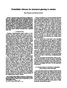
Figure 1: A typical transition graph (here for breakfast TV)

2. Modelling sequence structure using Markov Transition Graphs In this section we develop the Hidden Semi-Markov Model we will use later, starting with a relatively abstract model and showing how different ways of ‘concretising’ it lead to Hidden Markov Models and Hidden semi-Markov Models. We start with a sequence of observed feature vectors f1 , . . . , fT (eg, whole frames, block-correlation scores, etc) which are extracted from video of a physical scene where a particular behaviour is occurring. We have a set of states S={s1 , . . . , sS } (using superscripts to enumerate labels) corresponding to the various possible activity states occurring in individual frames. For the problem we deal with, at each timestep t the physical scene is in a particular state st , but we can’t compute st directly from ft , ie, the ss are hidden variables. This is due to observations containing a limited amount of information from the physical scene and, most intractably, imprecise models for scene understanding. However we assume we have observation models which compute the probability P (f|s) that feature vector f is observed when the system is in state s. The obvious way to get the most likely sequence of states is to pick the state with highest a posteriori probability for each frame independently. It’s clear, however, that if we have more knowledge about the system we can use this to perform more accurate inference. The most basic structure we can impose on the system is a transition graph such as Fig 1 describing allowed transitions between states, in this case derived from TV footage. At its most general, this graph specifies which new states are allowed when a state change occurs, thus allowing any interpretation where the sequence of states violates the graph to be discarded. A temporal process is called Markov when the future state depends only on the present state and not on the exact details of the past, for some chosen definition of ‘present’; the graph has the Markov property that the new state is constrained only by the present state. This is a trade-off: Markov assumptions enable efficient evaluation and, by limiting the number of model parameters, keep the amount of training data needed practical whilst captur-

ing the real world dependencies which are generally most significant. However, some natural constraints effectively cannot be expressed by a transition graph, a typical example being ‘moving to state Y can only occur if state X has occurred at some point in the past’. Nevertheless, for suitable problems the transition graph can be very effective. Models based on transition graphs. If, for each state si , we know the probability P (sj |si ) of each transition allowed by the graph, we could incorporate this into the inference process and thus compute a more accurate probability of a given interpretation. To complete this we have to handle remaining in the same state between adjacent timesteps. An obvious solution is to require a state transition at each timestep and add ‘transition to same state’ edges to the behaviour graph with appropriate probabilities; in terms of the Markov assumption this makes present mean ‘current frame’. The probability of observing features f1:T with interpretation s1:T is then P (f1:T , s1:T ) = P (s1 )

"

T Y

P (ft |st )

t=1

"

= P (s1 )P (f1 |s1 )

T Y

t=2

#"

T Y

t=2

#

P (st |st−1 ) (1) #

P (st |st−1 )P (ft |st ) (2)

= P (f1:T −1 |s1:T −1 )P (sT |sT −1)P (fT |sT)(3) where st is the particular state assigned at time t, a:b denotes a, . . . , b−1 and likewise xa:b =xa , . . . , xb−1 . (The prior probability of the initial state P (s1 ) complicates formulae and could be avoided with an artificial start state whose transition probabilities encode the prior on the true initial state.) This is the standard Hidden Markov Model (HMM) [19]. Eq 1 shows the split into feature- and transition-based terms, whilst Eq 2 & Eq 3 shuffle terms to highlight the Markov property that the state for the new frame depends only on the new observation, the state for the present timestep and the overall probability of the state sequence so far. One answer to the question ‘what should one use as the values for the hidden states s1:T when observation sequence f1:T is seen?’ is the sequence s1:T which maximises the probability P (f1:T , s1:T ) in Eq 1. This has the advantage over other answers that s1:T obeys the transition constraints embodied in the transition graph. The recursive structure of Eq 3 is useful because it can be seen that the maximum value of P (f1:T , s1:T ) in Eq 1 for a particular choice of sT −1 occurs for the choice of P (f1:T −1 |s1:T −1 )P (sT |sT −1 ) with maximal value. This means that standard dynamic programming techniques [1, 19] can be used to perform this maiximisation incrementally taking O(S 2 T ) time overall. This maximisation process is known as inference or decoding.

However there is one assumption in this model which is not immediately obvious. By direct calculation we can see that the prior probability of staying in state si for exactly τ steps is P (si |si )τ (1−P (si |si )). Thus in a HMM the self-transition probability is really a parameter which tunes the prior geometric distribution [5] over the time in the current state. (A range of geometric distributions are shown in Fig 2d.) There are many situations where this is a reasonable model, particularly if the observation frequency is close to the typical time in the state, but it is often desirable to have a model which allows specifying different temporal priors, particularly if the observation frequency is much higher than the typical time in state. This can be achieved by using an additional probability distribution P (t|s):=P (spent exactly t timesteps in state | state iss) (4) instead of adding the self-transitions. These are assumed to be full distributions with non-zero (but increasingly small) probabilities for arbitrarily large durations. The probability of a sequence of observations is then composed from the probabilities of the transitions, state durations and features. This model is called a Hidden SemiMarkov Model (HSMM) (also known as an explicit duration HMM) [8, 17] where the equivalent of Eq 2 is the joint probability of the observations and the division of the sequence into intervals in a given state, ie, s0 during τ0 :τ1 , . . . , sm during τm :τm+1 , P (f0:T , s0 during τ0 :τ1 , . . . , sm during τm :τm+1 ) "m #"m #"m # Y Y Y = P (si |si−1) P (fτi :τi+1 |si ) P (τi+1−τi |si) (5) i=1

i=0

i=0

= P (fτ0 :τ1 |s0)P (τ1−τ0 |s0) "m # Y × P (si+1 |si)P (fτi :τi+1 |si)P (τi+1−τi |si)

(6)

i=1

= P (fτ0 :τm |s0 during τ0 :τ1 , . . . , sm−1 during τm−1 :τm ) ×P (sm |sm−1)P (fτm :τm+1 |sm)P (τm+1−τm |sm)

(7)

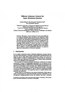
where “sm during τm :τm+1 ” means the system was in state sm from time τm to τm+1 − 1 and we require τ0 =1 and τm+1 =T . Again, Eq 5 expresses the probability in terms of the feature, duration and transition components taken separately. (There is an assumption here that the time-instate and observed features are independent given the state, which is often reasonable.) Similarly in Eq 6 & Eq 7 they have been shuffled to show the Markov structure, although now present means ‘current segment’. Models for state duration. The top row of Fig 2 shows a set of histograms of state duration for various classes obtained from the manually labelled ground truth (discussed

35

12 "class00.distrib"

30

mode. Consequently a gaussian is also a poor model and instead we model the time-in-state with a ‘modified gamma distribution’. This generalisation of the gamma distribution [5] parameterised by γ and β has pdf

0.9**x*0.1 0.8**x*0.2 0.7**x*0.3 10

25 8 20 6 15 4 10

2

5

0 0

20

40

60

80

100

p(t) = (t/β)γ exp(−(t/β)z )/Z

0 140 -10

120

-5

(a)

0

5

(d)

30

0.2 "class01.distrib"

0.4*exp(-(x-5)**2/2)/2 0.4*exp(-(x-5)**2/4)/4 0.4*exp(-(x-5)**2/8)/8

0.18 25 0.16 0.14 20 0.12 15

0.1 0.08

10 0.06 0.04 5 0.02 0 0

20

40

60

80

100

120

140

0 160 0

2

(b)

4

6

8

10

(e)

50

0.35 "class02.distrib"

(x/2)**2*exp(-(x/2)**1.1)/2.87 (x/2)**3*exp(-(x/2)**1.1)/6.6109 (x/2)*exp(-(x/2)**1.1)/1.0614

45 0.3 40 0.25

35 30

0.2 25 0.15 20 15

0.1

10 0.05 5 0 0

2

4

6

8

10

12

(c)

14

16

18

0 20 0

2

4

6

(8)

10

8

10

(f)

Figure 2: (left) histograms of time-in-state; geometric; (right) geometric, gaussian & modified gamma distributions

below). These have a rough characteristic shape where the probability of a given duration rises quickly to a most likely duration, then tails off significantly more slowly, a poor fit with the set of shapes obtained with a geometric distribution. The obvious approach is to model the duration distribution using an empirical histogram. However, because each sample comes from a segment comprising perhaps tens of frames obtaining sufficient training data to adequately populate the histogram is difficult. Although we could try histogram smoothing, we choose instead to model the distribution with a parametric distribution. Two advantages are that we automatically generate a smooth distribution from the data and can accommodate prior knowledge about the likely time-in-state via priors on the parameters. We argue that using a roughly appropriately shaped parametric distribution is acceptable when training data is limited, even though we don’t know if the ‘true’ generating distribution is in the chosen family. (An argument could be made for possible multi-modality in these distributions, which might suggest a mixture model, but with at most 100–200 examples per class – from a 12,500 frame ground truth – a meaningful conclusion cannot be drawn about this.) To choose the parametric family, observe that the timein-state is restricted to positive values and the empirical distributions in Fig 2 are noticeably asymmetric around the

where z is some constant >1 and normalizing constant Z is equal to βΓ( γ+1 z )/z. (As we use different distribution parameters for each state s the normalising constants do not cancel.) The plots in Fig 2 show examples of geometric, gaussian and modified gamma distributions; it is clear that the modified gamma is the most similar to the empirical plots. Fitting parameters given training data is complicated since even with 100–200 examples there are still areas of low sample density and wide variation between adjacent time points. Although we attempted to fit distributions automatically, the restricted number of samples resulted in curves distorted by the requirements of fitting against the inadequately sampled right-hand tails of the histograms; consequently we fitted appropriate looking distributions manually for our experiments. More extensive ground truth datasets would enable automatic fitting of the distributions.

3. Computing the most likely HSMM decoding of a sequence The activity recognition process is formulated as finding the most likely sequence of states according to the HSMM parameters. An O(S 2 T 2 ) HSMM most-likely sequence inference algorithm which works with arbitrary duration distributions is given in [17]. This time complexity essentially arises because at each timestep a maximisation has to be performed not only over all states for the previous timestep but also all possible lengths of time in that state. This quadratic behaviour is infeasible when working with long video sequences (large T ), so we develop an O(S 2 T ) algorithm (adapting [11]) by first showing the key step in inference is deciding between different segmentations ending at the same time, then show how this can be tackled effectively using structure within the HSMM model. HSMM inference as optimal segmentation. For the standard HMM the natural view of inference is that of assigning states at each time, whereas for the HSMM inference is most naturally viewed as segmenting the sequence into intervals with a common state. We want to find the best division into segments using an algorithm which is recursive in that the optimal segmentation of a sequence can be computed using the optimal divisions of its prefixes. In a similar way to the standard HMM algorithm at each time t we find, for each state s, the best segmentation which ends in state s at t. The Markov property of the HSMM means that the

time a

time b

time t−1

τ

time t+t’

state s state s’

a

state s’’

Figure 3: two potential segmentations, both of which transition to a final the same final state s only influence from the previous segments comes from the total probability of that previous state and the time at which the transition to the present state occurred. This is illustrated by Fig 3, where the top line indicates the timeline in state s, whilst the other two lines show two segmentations which switch to s for the final block. The dashed segments on the left indicate the best probability previous segmentations (where we will see below the exact details of which don’t matter). So the basic task is to decide between two such segmentations, both of which finish in a segment in state s at time t−1. Structure in HSMM probabilities. We will show that, with a standard ‘naive Bayes’ assumption on feaQ tures P (fa:b |s) = b−1 i=a P (fi |s), which of two segmentations ending in s is best doesn’t depend on the feature data in their common suffix. To do this we compare the probabilities of two hypothesised segmentations which have the common feature of both finishing at time t−1 in a segment in state s. (A schematic illustration shown in Fig 3.) In one case this final segment begins at time a with and has a probability Ph1 =P (f1:a |to a) for a hypothesised segmentation to a for the initial sequence f1:a . (Fig 3 shows the previous history before the transition being in a state s0 but the key point is that the only factor affecting the calculations is the probability P (f1:a |to a)). We have a second sequence which transitions to s at time b (where a0 and arbitrary constants C1 and C2 . This intuitively states that ‘given two segmentations ending in the same state at a common time, once they have been extended with new frames’ data until the longer segmentation has a lower probability, then it will always have a lower probability as both segmentations are further extended over the feature sequence’. If we keep track of candidate segmentations and

5

initialisation 1 2

for s∈S: #initialise each queue with one big interval set q[s]:=hri with r.nlp:=0, r.t0 :=1 & r.dom int st:=1

main algorithm #build up the best solution recursively for t:=1, . . . , T : 4 for s∈S such that t≥q[s].hd.next.dom int st: 5 pop head(q[s])#discard intervals as time passes domination point 6 for s∈S: #figure what’d happen if sequence ends in state s 7 create r with r.nlp:=∞ #make r ‘impossibly unlikely’ 8 for s0 ∈S\{s}: #find best transition from other state into s at time t 9 add −logp(ft |s0 ) to .nlp of each entry on q[s0 ] 10 q[s0 ].hd.nlp:=sum of old nlp, duration & transition values 11 if q[s0 ].hd.nlp