Hindawi Publishing Corporation International Journal of Distributed Sensor Networks Volume 2014, Article ID 386982, 14 pages http://dx.doi.org/10.1155/2014/386982
Research Article Efficient Image Transmission over WVSNs Using Two-Measurement Matrix Based CS with Enhanced OMP Hemalatha Rajendran, Radha Sankararajan, and Jalbin Justus Department of Electronics and Communication Engineering, SSN College of Engineering, Kalavakkam, Chennai 603110, India Correspondence should be addressed to Hemalatha Rajendran;
[email protected] Received 7 June 2013; Revised 1 October 2013; Accepted 30 October 2013; Published 5 January 2014 Academic Editor: Hongkai Xiong Copyright © 2014 Hemalatha Rajendran et al. This is an open access article distributed under the Creative Commons Attribution License, which permits unrestricted use, distribution, and reproduction in any medium, provided the original work is properly cited. WVSN is a collective network of motes containing visual sensors. The nodes in the network are capable of acquiring, compressing, and transmitting successive images to the sink. To increase the lifetime of such network, it is essential to reduce the amount of dataflow across the network without losing the integrity. This paper proposes a CS-based image transmission system to reduce the number of measurements required to represent the image. It utilizes a two-measurement matrix-based CS. TMM with CS leads to 2.8% to 6.7% and 0.67% to 7.9% reduction in the number of measurements compared to one MM-based CS while using DCT and binary DCT, respectively. Similarly, TMM with NUS CS leads to 5% to 40% (DCT) and 1.4% to 20% (binDCT) reduction in the number of measurements than one-measurement matrix-based NUS CS. An Enhanced Orthogonal Matching Pursuit algorithm is also proposed, which produces nearly 2% to 26% better recovery rate with the same number of measurements than the conventional OMP algorithm. Reduced measurements and better recovery rate achieved will enhance the lifetime of the WVSN, with considerable image quality. Rate distortion analysis of the proposed methodology is also done.
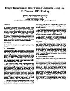
1. Introduction WVSNs are networks of wirelessly interconnected devices equipped with camera, enabling the retrieval of video and audio streams, still images, and scalar sensor data. They have tiny visual sensor nodes called camera nodes as shown in Figure 1, which integrate the image sensor, embedded processor, and wireless transceiver [1]. WVSNs have large volume of data to be processed and stored which increases the complexity of the system. With the advancement in the image sensor technology, WVSNs can be used for more complex multimedia applications like border surveillance using visual monitoring, tracking rare animal species, controlling the vehicle traffic on highways, and railways and environmental monitoring [1–3]. However, they are energized by small batteries with a short span of lifetime. Replacing or recharging of the battery is also extremely difficult. With reduced lifetime of the batteries image transfer application in WVSNs has the limitations such as reduced bandwidth, reduced on board memory,
and limited computational capability. Hence, it is essential to aim at diminishing the amount of data to be processed and the level of computations involved. WVSNs are in need of a compression process with acceptable compression rate, low computational complexity, low power consumption, and low dynamic memory usage to reduce the number of bits used for representing the image, which will also reduce the communication cost of the bits to be sent to the destination. Conventional image compression algorithms convert high-resolution images into a relatively small bit streams, in effect converting a large digital data set into a substantially smaller one. Eventually, data compression can be built directly into the acquisition process using CS. CS is used to recover a sparse signal from a less number of linear measurements. An image which is compressible in some basis can also be reconstructed perfectly from a small number of linear measurements [4]. The three inherent inefficiencies of traditional image compression techniques are as follows:
2
International Journal of Distributed Sensor Networks
Sink Event
Camera mote
Figure 1: Visual sensor network architecture [1].
(i) initial number of samples “𝑝” may be large even if the desired number of samples “𝑏” is small; (ii) set of all “𝑝” transform coefficients must be computed even though we need only “𝑏” of them; (iii) locations of the “𝑏” transform coefficients must be encoded. CS overcomes these inefficiencies by directly acquiring a compressed signal representation without going through the intermediate stage of acquiring “𝑝” samples [4, 5]. Consider a real valued, finite length, one-dimensional signal 𝑋 ∈ 𝑅𝑁. Using the 𝑁 × 𝑁 basis matrix 𝜓 = [𝜓1 | 𝜓2 | ⋅ ⋅ ⋅ | 𝜓𝑁] with the vectors {𝜓𝑖 } as columns, a signal 𝑋 can be expressed as 𝑁
𝑋 = ∑ 𝑆𝑖 𝜓𝑖 = 𝜓𝑆,
(1)
𝑖=1
where 𝑋 is 𝑁 × 1 column vector with coefficients 𝑋𝑖 , 𝑖 = 1, 2 . . . 𝑁 and 𝑆 is vector of coefficients representing 𝑋 in 𝜓 basis. The process of measurement in CS [5] can be defined as 𝑦 = 𝜙𝑋 = 𝜙𝜓𝑆 = Θ𝑆,
(2)
where 𝜙 is an 𝑀 × 𝑁 random matrix, Θ = 𝜙𝜓, 𝑋 is a 𝑁 × 1 sparse coefficient input vector, and 𝑦 is a 𝑀 × 1 measurement vector. It is assumed that 𝑀 < 𝑁. The number of measurements depends upon the sparsity and incoherence [6, 7]. Low coherence between measurement basis 𝜙 and representation basis 𝜓 results in a less number of measurements. The number of measurements 𝑀, for perfect reconstruction of a 𝑧-sparse 𝑁-dimension signal [6] is given by 𝑀 ≥ 𝛼 ⋅ 𝑧 ⋅ log (
𝑁 ), 𝑧
(3)
where 𝛼 is some positive constant affecting the probability of recovery. Signal 𝑋 could be recovered exactly by solving the minimum l1-norm optimization problem. The reconstruction process is formulated as 𝑆̂ = min‖𝑆‖ℓ1 𝑆
̂ subject to 𝑦 = Θ𝑆, 𝑋 = 𝜓𝑆.
(4)
This methodology can be made in-built during the acquisition process itself. Hardware realization is available in [8]. Since it is still in research, CS-based compression is proposed expecting the availability of hardware in the near future. The whole image is taken as the input and analysed how better it could have been captured with CS as in [5]. CS requires the choice of the measurement matrix (MM), recovery algorithm, and the sparsity basis. It reduces the data in hand on the initial stage itself, which will surely reduce the computational complexity and storage requirement burdens evolving in the WVSNs scenario. This motivated us to propose a scheme combining the CS and WVSNs to get better efficiency for the image transmission applications. The proposed scheme provides better recovery rate and acceptable image quality with much reduced number of measurements. The rest of the paper is organized as follows. Section 2 provides the brief review of the related work. Section 3 discusses the system model that is proposed in detail. Section 4 presents the performance evaluation based on the number of measurements, percentage of recovery, Peak Signal to Noise Ratio (PSNR), and Bpp, and Section 5 gives the conclusion.
2. Related Work Romberg [5] proposed a compressive imaging technique using both DCT and Noiselet coefficients. The algorithm is applied for the entire image; the measurement includes the DCT elements taken after zigzag ordering used in JPEG and random Noiselet measurements. It provides better image quality, but the random locations of the Noiselet coefficients have to be conveyed to the receiving end for proper recovery. The recovery is done using optimization technique by reducing the total variation. It is time consuming and very complex. Sermwuthisarn et al. [9] divided the image into blocks and used Haar wavelets as sparse basis. The measurements are taken using Noiselet MM. Though the block based processing provides low memory and low-computing time, the sparsity varies from block to block so the MM size also changes. So, the details of the MM have to be sent along with the measurements which will also increase the energy consumption in case of WVSNs. Tsaig and Donoho [10] explored that CS can
International Journal of Distributed Sensor Networks be applied in a different way in image recovery. CS is applied to measure only fine scale properties of the signal, while ordinary linear measurement and reconstruction were used to obtain the coarse-scale properties of the signal. It provided better image quality. Zhou et al. [11] proposed NUS of CS. The image is divided into blocks, DCT transformed, zigzag ordered, and then classified as important and nonimportant coefficients. Important coefficients are transmitted as such and the CS measurements are taken over the nonimportant coefficients. Though it provides better quality with reduced measurements, it has increased complexity and MM changes from block to block further increasing the burden. Alternatively, a methodology using TMM by identifying the blocks to be low-frequency content block or high-frequency content block based on the number of nonzero elements is proposed. This is the extended version of the one proposed in [12] and is utilized in both CS and NUS measurement strategies, enabling efficient implementation in WVSNs. The measurements are taken using binDCT also, which reduces the energy consumption of the entire process, whereas in [12], only DCT is used. EOMP recovery algorithm is used in this paper to get better recovery rate while in [12] OMP is used. This reduces the number of measurements and the complexity. CS enables the recovery of the sparse signals from a relatively small number of linear measurements. This requires the incoherent nature of the MM with the sparsity basis. There are many existing contributions that model and propose the MM generation. Cand`es et al. [6] used Gaussian random matrix which has inherent restricted Isometry property. Cand`es and Romberg [7] utilized the nonbinary orthogonal transform matrices as MM. They have fast transform algorithms, for example, Scrambled Fourier (SF) matrix. But these matrices have non binary element, which is a major drawback, hence the hardware implementation will be difficult in these cases and multiplication is done to take the measurements. Multiplications in the on-board processors of the mote will consume much energy. Sparse matrices generated from block diagonal matrices, Scrambled Block Hadamard (SBH) [13], and Binary measurement matrices [13, 14] are available in the literature, but they are computationally complex to be implemented in WVSNs. As an alternative, we have taken a binary sparse matrix with uniform distribution. Hence, the measurement process involves only additions. Recovering the sparse signals from reduced number of measurements is an NP-hard problem. The two major algorithmic approaches to sparse recovery are based on L1-minimization and iterative methods (Matching Pursuits). The optimization techniques use either convex or linear programming to solve the L1 problem in it. But their implementation is very much time consuming and very complex [15]. The greedy algorithms use the correlation between the signal and the columns of the MM as a measure to find the elements with nonzero coefficients. There are several such algorithms [16– 22] in the literature. In this paper, we concentrated on the matching pursuit algorithms due to its simple and fast implementation. Tropp and Gilbert [16] proposed the OMP algorithm in which the sparse signal is recovered by choosing a strong correlated column of the MM in each iteration and
3 the contribution of chosen column is subtracted from the measurements. The original signal is recovered after 𝑧 (sparsity level) number of iterations. Its advantage is fastness and transparency. But OMP has weaker guarantees of exact recovery. Needell and Vershynin [17] suggested ROMP, where 𝑧 biggest columns of the MM are chosen and are regularized with the maximal energy concept. It terminates in at most 2𝑧 iterations. The disadvantage is that finding the least squares solution in each iteration is tedious with more number of columns being included in the support set. Baby and Pillai [22] proposed ordered OMP, an improvement to OMP. The wrongly detected columns in the support set are removed by comparing the projection coefficients and are scaled down to avoid the reentry. It achieves exact recovery at a smaller number of measurements when compared to OMP. Our work is to decrease the number of measurements for exact recovery with reduced complexity. Hence, we propose the EOMP algorithm for recovery with two column entries into the support set in each iteration, with wrong column detection and its suppression. The elements of the support set are checked to get rid of duplications in the successive iterations. It provides exact recovery at very lesser measurements. The performance of the proposed algorithm is evaluated and compared with the OMP [16], ROMP [17], and OOMP [22]. Haupt et al. [23] have done a decentralized compression of networked data using CS. Yu et al. [24] have used CS to remove the redundancy in spatially neighbouring measurements, in the Vehicular Sensor Network (VSN). CS provides accurate reconstruction and less communication load for surveillance and urban monitoring applications. Mamaghanian et al. [25] have utilized CS for low-complexity energy-efficient ECG compression. The lifetime of the network is increased in all CS-based WSN applications [23–25]. Hence, this paper proposes an image transmission methodology using CS in WVSNs to prolong its lifetime. BinDCT [26, 27] is suggested for the transformation of the image in NUS strategy (hybrid CS). This will reduce the power consumption of the on board processor in the WSN mote. Measurements are taken using TMM procedure with binary valued MM to reduce the number of measurements required for the recovery of an image with acceptable quality. Encoding is done using the JPEG Huffman table. Reconstruction algorithm is improved to provide better performance. It gives exact recovery at very much less number of measurements. This reduces the number of measurements transmitted from the source to the destination. This paper mainly aims at the reduction of the number of measurements and to provide better recovery rate. This will increase the lifetime of the network, the foremost requirement in the real time applications.
3. Proposed System Model The proposed CS-based compression algorithm for the WVSN is shown in Figure 2. The processes shown in the transmitter section will take part in the visual sensor nodes and the recovery as in the receiver section will be done at the powerful information collecting node called sink.
4
International Journal of Distributed Sensor Networks Table 1: Comparison of DCT methods used for 8 × 8 matrix.
CS measurements using TMM
Input image
CS measurements using TMM
Block division
Compressed image Encoding
Type Floating Point DCT Integer DCT Chen-C1
CS measurements using TMM
No. of multiplications
No. of additions
No. of shifts
1024
896
—
—
672
368
(a) Transmitter section
Reconstructed Block combiner image
Inverse DCT/ BinDCT
Enhanced OMP
Inverse DCT/ BinDCT
Enhanced OMP
Inverse DCT/ BinDCT
Enhanced OMP
Compressed image Decoding
TMM: two measurement matrix
(b) Receiver section
Figure 2: Proposed system model.
The captured input image is divided into a block of size 𝑠 × 𝑠 and spatially transformed using binDCT. DCT is chosen since it has high energy compaction property. Block size is chosen as 𝑠 = 8, so that it reduces the blocking artefacts and blurring effect in the reproduced image. It also considerably reduces the memory requirement for MM storage essential to take the CS measurements. The measurement matrix size is 𝑀 × 64 (𝑀 × 𝑠2 ). The further increase in the block size will drastically increase the size of MM and its storage requirement. Hence, we fixed the block size to be 8. Binary DCT is applied on the blocks to get the transformed image and to sparsify the image in NUS strategy. The conventional floating point method of computing DCT is very exhaustive. The floating point method computes the DCT using multiplications and additions. The energy consumed for multiplications is generally high when compared to additions or shifting operations. As we have a limited power supply at the source node, it is important to utilize it effectively. On this regard, we use the concept of binDCT to replace the floating point DCT. Using binDCT, the forward and the inverse transforms are implemented using only binary shift and addition operations. The energy consumed via this method would be far less than the conventional method. There are several families of such multiplierless binDCT computations. The configuration employed in this work is that of C1-Chen’s factorization [26]. Comparison of the operations involved in the conventional method and binDCT method is listed in Table 1. The transformed image is converted into a column vector (𝑥). To sparsify “𝑥”, only 𝐷% of “𝑥” is kept and other elements are made to be zero. Choice of the 𝐷 is made based on the quality requirement of the reconstructed image. The measurement procedure is described in detail in Section 3.
The measurements are encoded using the conventional JPEG Huffman table [28]. The coded data is transmitted to the sink. At the sink, the received data is decoded and then the recovery is done through the proposed EOMP algorithm briefed in Section 4. It enables the reconstruction of the image with much reduced measurements compared to the conventional algorithms [7, 16, 22]. The reconstructed column vector is converted into a matrix of size 8 × 8 and inverse binDCT is applied. Then, the blocks are arranged properly to get back the reconstructed image. The procedure is also repeated with DCT transformation. Here, two-level compression is done to get better compression rate as follows. (i) The required measurements to represent the image are reduced by CS. (ii) The redundancy in the measurements is removed by encoding it using the standard JPEG Huffman table. The entire process is formulated to reduce the computational complexity, the amount of data to be processed and transmitted, and the storage requirements (memory). The main reduction in the processing data is achieved due to the CS-based TMM techniques and EOMP algorithm. 3.1. Two-Measurement Matrix-Based CS. When an image is divided into blocks of small size, the frequency component in each block will not be the same. A block with smooth variations in the gray level contains only few large amplitude DCT coefficients. It is called as the low frequency component of the image. A block with sharp variations in the gray level contains more large amplitude DCT coefficients. It is called as the high frequency component of the image. This is shown in the cameraman image in Figure 3. The block 1 is one of the low frequency content blocks and it has only one large amplitude DCT coefficient. The block 2 is one of the high frequency content blocks and it has approximately 28 large amplitude DCT coefficients. If same-sized MM is used to measure both low-and highfrequency content blocks, it results in a large number of measurements. The proposed method uses two measurement matrices with different sizes. The MM with large number of rows is used to measure the high frequency content blocks and the MM with less number of rows is used to measure the low frequency content blocks, thereby reducing the total number of measurements. Based on the application (e.g., object detection) the number of measurements can be further reduced by sacrificing the quality of the image. In WVSNs, bandwidth is a constraint, which is solved by the proposed
International Journal of Distributed Sensor Networks
5 Input image
Block 1
Block division
DCT/BinDCT Block 2
Single column vector
Important component
Unimportant component (X)
Is it low frequency content component?
Yes
Figure 3: Example of low-frequency and high-frequency blocks.
y = 𝜙1 𝜓X
No
Side information (1/0)
y = 𝜙2 𝜓X
Encoder
For each block in a image (1) Convert to a column vector 𝑥 of size 64 × 1. (2) Quantize: 𝑥𝑞 = 𝑥/2𝑛 , 𝑛 = 1, 2, 3 . . . (3) Find the number of nonzero elements 𝑁nz (4) Compare 𝑁nz with a pre-fixed threshold (𝑇) and set the sparsity level 𝑆 if 𝑁nz > 𝑇 SL = ℎ 𝑆𝑙 if 𝑁nz < 𝑇 (5) Sparsify 𝑥𝑞 to have SL nonzero elements. (6) Generate 𝜙 (MM) of size (SL ⋅ log (64)) × 64 (7) Take linear measurements, 𝑦 = 𝜙𝑥𝑞 Algorithm 1
Important component
Measurements
Decoder
Side information Check 1/0
1 𝜙1 𝜓
0 𝜙2 𝜓
Enhanced OMP
Rearrangement
method, which produces less number of measurements. The procedure for the TMM allocation is summarised in Algorithm 1. This variation leads to reduction in measurements since the nature of the image is exploited to take measurements. 3.2. Two-Measurement Matrix-Based Nonuniform Sampling CS. In nonuniform sampling-based CS, transformed coefficients in each block are separated into important and unimportant component [11]. Important components are the first few elements taken after zigzag ordering the block. They are transmitted as such, whereas the remaining unimportant components undergo CS measurement. If same measurement matrix is used to measure the unimportant component of all blocks of an image (i.e., the unimportant component of lowfrequency content blocks and high-frequency content blocks are weighted equally), it results in a large number of measurements. The proposed method uses two measurement matrices in nonuniform sampling-based CS as shown in Figure 4.
Inverse DCT/BinDCT
Rearrange blocks
Estimated image
Figure 4: Flow chart of the proposed two measurement matrixbased nonuniform sampling CS.
The measurement matrix with large number of rows is used to measure the unimportant component of high frequency content blocks (𝜙1 ) and the measurement matrix with less number of rows is used to measure the unimportant component of low frequency content blocks (𝜙2 ), thereby reducing the total number of measurements. The size of important component of all blocks is kept as constant.
6
International Journal of Distributed Sensor Networks
Input: (i) An 𝑀 × 𝑁 measurement matrix 𝜙. (ii) An 𝑀-dimensional measurement vector 𝑦. (iii) The sparsity level 𝑧 of the ideal signal. Procedure: Step 1. 𝑟0 = 𝑦, Λ 0 = 0 and the iteration counter 𝑡 = 1. Step 2. Find the index 𝜆 𝑡 that solves the easy optimization problem. 𝜆 𝑡 = arg max𝑗=1,2... 𝑁 ⟨𝑟𝑡−1 , 𝜑𝑗 ⟩ Step 3. Augment the index set Λ 𝑡 = Λ 𝑡−1 ∪ {𝜆 𝑡 } and the matrix of chosen atoms. 𝜙𝑡 = [𝜙𝑡−1 𝜑𝜆𝑡 ⌋ Step 4. Solve the least-square problem to obtain a new signal estimate. 𝑔𝑡 = arg min𝑔 𝜙𝑡 𝑔 − 𝑦2 Step 5. Calculate the new approximation of the data and the new residual. 𝑎𝑡 = 𝜙𝑡 𝑔𝑡 , 𝑟𝑡 = 𝑦 − 𝑎𝑡 Step 6. Increment 𝑡 and return to Step 2 if 𝑡 < 𝑧. ̂ for the ideal signal has non-zero Step 7. The estimate 𝑋 indices at the components listed in Λ 𝑧 . The value of the ̂ in component 𝜆 𝑗 equals the 𝑗th component of 𝑔𝑡 . estimate 𝑋
Algorithm 2: OMP [16].
The important component is transmitted to the receiver directly along with CS measurements of unimportant component. The measurement matrices are assumed to be known to the transmitter and receiver. One extra bit (side information) per block is transmitted to inform the receiver which measurement matrix is being used for that block. The unimportant component is estimated at the receiver by using EOMP algorithm. Then important component is concatenated with it. Then, the resultant single column vector is rezigzag ordered to form a matrix. Then, inverse transformation is applied to this matrix to get the estimated block. These blocks are rearranged to form the estimated image. Both DCT and binDCT transforms are applied for analysis. 3.3. Recovery Enhanced OMP. The proposed recovery algorithm is a modification of the OMP [16]. Though there are several recovery algorithms [18–21], OMP is very popular due to its low computation cost and its ease of implementation. The main idea of the OMP is to pick the highly correlated column with the received signal. The index of the same is also accumulated in a counter Λ consecutively. Signal estimate is found using the least squares solution with the available column set. The contribution of the support set is removed from the residue to maintain orthogonality between the residual and the support set. Hence, the algorithm discovers new column in each iteration. This column usually corresponds to the largest coefficient of the sparse signal. But at some instances, OMP fails to pick up the correlated columns correctly. So, it needs more measurements to ensure exact recovery. Algorithm 2 explains the procedure involved in OMP.
In this paper, the falsely selected columns are identified in each iteration and are removed from the support set. The approximation coefficients as in step 4 can also be found by −1 𝑔𝑡 = (𝜙𝑡𝑇 𝜙𝑡 ) 𝜙𝑡𝑇 𝑦. It is the projection of 𝑦 on to the subspace spanned by the columns in 𝜙𝑡 . The projection coefficients are used to check whether a column in the present support set is falsely detected or not. To check the false detection, two parameters are included as follows: (i) acceptance range, 𝜀 < 1, (ii) suppression factor, 𝛼 < 1. In every iteration, EOMP compares the projection coefficients with that obtained in the previous iteration. A column in the present support set is declared as wrongly detected if its present projection coefficient falls below 𝜀 times, its value in the previous iteration. If any column fails this test, that is, if its coefficient gets smaller, then that column will be removed from the support set. Furthermore, that column is scaled down by 𝛼 so that the column is given less importance in the coming iterations. Algorithm 3 explains the EOMP algorithm. In the proposed algorithm after calculating the first estimate, two highly correlated columns are included in the index set. If there is any duplication, it will be removed. Then, the current estimate is compared with the previous estimate, if it is up to the expected significant level, then the column identification is correct, if not the columns are taken as false identifications. The false columns will be removed from the submatrix, their contribution is subtracted from the residual. They are also suppressed by a factor of 𝛼. The algorithm tries to find the best approximation for the estimated input vector rather than relying on the highly correlated values. Acceptance range (𝜀): it is used to find the wrongly detected columns, as their entry will reduce the projection coefficient values. If the current estimate value is less than 𝜀 times the previous estimate at one or more locations, then those entries are assumed to be wrong and are removed from the support set. Suppression factor (𝛼): this factor is used to suppress the wrongly detected columns from again entering into the support set. It enables easy convergence towards the correct support set. To get better result, the accurate choice of the above mentioned factors is essential. It depends on the sparsity and size of the input vector. The values adopted for the image transmission are explained in Section 4.
4. Performance Evaluation The proposed CS-based image transmission is implemented using EOMP algorithm and TMM technique. Performance metrics like percentage of recovery and PSNR are calculated and compared with OMP, ROMP, and OOMP. The proposed EOMP has better performance with the same level of complexity. The entire transmission algorithm is compared with the single measurement matrix method using OMP. The proposed technique requires less number of measurements to ensure the same level of PSNR than the existing one. The
International Journal of Distributed Sensor Networks
7
Input: (i) An 𝑀 × 𝑁 measurement matrix 𝜙 (ii) An 𝑀-dimensional measurement vector 𝑦 (iii) The sparsity level 𝑧 of the ideal signal and the sparsity basis. (iv) Acceptance Range, 𝜀 and suppression factor, 𝛼 Procedure: −1 Step 1. Find 𝜆 1 = arg max𝑗=1,2,..,𝑁 ⟨𝑦, 𝜑𝑗 ⟩, Λ 1 = {𝜆 1 }, 𝜋 = ⌊𝜑𝜆 ⌋, 𝑔1 = (𝜋𝑡𝑇 𝜋𝑡 ) 𝜋𝑡𝑇 𝑦, residual, 1 𝑟1 = 𝑦 − 𝜋𝑔1 Step 2. iteration counter 𝑡 = 2, 𝑘 = 1. Set values for 𝜀 and 𝛼. While 𝑘 ≤ 𝑧, do Step 3. Find ⟨𝑟𝑡−1 , 𝜑𝑗 ⟩ 𝑗 = 1, 2, . . . , 𝑁. Take two maximum correlated indexes 𝜆 𝑡 = {𝜆 ℎ1 𝜆 ℎ2 } Step 4. Augment the index set Λ 𝑡 = Λ 𝑡−1 ∪ {𝜆 𝑡 } and the sub-matrix of chosen atoms 𝜙𝑡 = [𝜙𝑡−1 𝜑𝜆𝑡 ⌋ where 𝜙0 is an empty matrix. /Two element entry/ Step 5. If there is any duplications in the index set, remove it by emptying the corresponding index. Remove the atom in the sub-matrix also. /Duplication removal/ Step 6. Find a new signal estimate: 𝑔𝑡 = arg min𝑔 𝜙𝑡 𝑔 − 𝑦2 /Wrong index detect / Step 7. For 𝑖 = 1, 2, . . . , 𝑧, if 𝑔𝑡 (𝑡 − 𝑖) ≤ 𝜀 𝑔𝑡−1 (𝑡 − 𝑖) for some 𝑖 = 𝑗, then (a) Λ 𝑡 = Λ 𝑡 − {Λ 𝑡 (𝑗)}, 𝜙𝑡 = 𝜙𝑡 − {𝜙𝑡 (𝑗)}, /Wrong index removal/ /Residue updating/ (b) 𝑔𝑡 = arg min𝑔 𝜙𝑡 𝑔 − 𝑦2 /Suppressing Re-entry/ (c) 𝜑Λ 𝑡 (𝑗) = 𝛼𝜑Λ 𝑡 (𝑗) Step 8. Update the residue vector: 𝑎𝑡 = 𝜙𝑡 𝑔𝑡 , 𝑟𝑡 = 𝑦 − 𝑎𝑡 Step 9. Increment 𝑡, 𝑘 and end while Algorithm 3: EOMP.
4.1. Recovery Enhanced OMP. The working of the EOMP mainly depends on the choice of the parameters 𝜀 and 𝛼. The effect of suppression factor is analyzed first. Sparsity is fixed as 4 and acceptable range 𝜀 is taken as 0.5 and the 𝛼 value is changed from 0.05 to 0.95; the corresponding percentage of recovery is plotted in Figure 5. For each value of 𝛼 the number of measurements is varied from 0 to 64. Percentage of recovery is averaged over 1024 independent trials of the data set 𝐷(𝑧, 𝑀, 𝑁). From Figure 5, it is evident that variation in 𝛼 did not affect the percentage of recovery. The change is less than 1% for all the cases; hence, all the curves are overlapped. So, 𝛼 value can be chosen independently from the range 0.05 to 0.95 as it has not much influence on the percentage of recovery. The percentage of success for a fixed measurement remains almost the same for the entire range of variation of the 𝛼 and hence 𝛼 can have any value between 0.05 and 0.95 as shown in Figure 6. The same is checked for different sparsity levels also. The effect of the acceptance range is studied with 𝛼 = 0.7, 𝑁 = 64 and the sparsity takes the following values 𝑧 = 2, 6, 10. The acceptance range is varied from 0.05 to 0.95 for all the individual cases. The percentage of recovery is calculated and
100 90 80 Percentage of recovery
entire simulation is done using Matlab (R2011a). The data set 𝐷 (𝑧, 𝑀, 𝑁), having an ensemble of random matrices 𝜙 of size 𝑀 × 𝑁 and an ensemble of 𝑧 sparse vectors is considered. The length of the data vector (𝑁) is fixed as 64, since the block size of 8 is chosen in the processing of the image. Sparsity and the measurements are varied and the results are analysed.
70 60 50 40 30
20 10 0
0
10
20 30 40 50 Number of measurements
60
70
Figure 5: Percentage of recovery for 𝛼 varied from 0.05 to 0.95 with 𝑧 = 4, 𝜀 = 0.5, 𝑁 = 64.
is averaged over 1024 independent trials and is shown in Figure 7. The black, red, brown, green, and magenta curves correspond to 𝜀 = 0.75, 0.8, 0.85, 0.9, and 0.95, respectively. For 𝜀 = 0.05 to 0.7, the curve is plotted in blue color. In Figure 7(a), the response for 𝜀 = 0.05 to 0.7 does not have much variation in terms of the percentage of recovery. So, the lines get overlapped and are visible as a single line, whereas the percentage recovery starts decreasing when the 𝜀 value is increased beyond 0.7. With the increase in 𝜀, the checking limit for the column to be identified as wrong detection is
8
International Journal of Distributed Sensor Networks 100
Percentage of recovery
95 90 85 80 75 70
0
0.2
0.4
0.6
0.8
1
Alpha z=2
z=6 z=4 100
90
90
80
80 Percentage of recovery
Percentage of recovery
Figure 6: 98% of recovery for 𝛼 variation from 0.05 to 0.95 with 𝑁 = 64. 100
70 60 50 40 30
70 60 50 40 30
20
20
10
10
0
0
10
20
30
40
50
60
0
70
0
Number of measurements
0.5–0.7 0.75
0.8 0.85
10
20 30 40 50 60 Number of measurements
0.5–0.7 0.75
0.9 0.95
(a) 𝑧 = 2
0.8 0.85
70 0.9 0.95
(b) 𝑧 = 6
100 90
Percentage of recovery
80 70 60 50 40 30 20 10 0
0
10
20 30 40 50 60 Number of measurements 0.8 0.85
0.5–0.7 0.75
70
0.9 0.95
(c) 𝑧 = 10
Figure 7: Percentage of recovery of EOMP for 𝜀 varying from 0.05 to 0.95.
tightened. Hence, correct columns can also be identified as the wrongly detected ones, this leads to the performance degradation for the values of 𝜀 > 0.7. This holds good for the varying values of the sparsity also, which is shown in Figures 7(b) and 7(c).
In all the cases, system becomes unstable or has degraded performance for 𝜀 > 0.7. Hence, we omitted the range above 0.7 for 𝜀. In the range of 0.05 to 0.65, any value can be chosen since there is no drastic degradation in the performance when 𝑧 = 2, but when sparsity increases, 𝜀 = 0.65 and 0.6 has
International Journal of Distributed Sensor Networks
9
100 90
Percentage of recovery
80 70 60 50 40 30 20 10 0
0
10
20
30
40
50
60
70
Number of measurements EOMP, z = 2 OMP, z = 2
EOMP, z = 4 OMP, z = 4
EOMP, z = 6 OMP, z = 6
100
100
90
90
80
80
70
70
Percentage of recovery
Percentage of recovery
Figure 8: Comparison of OMP and EOMP.
60 50 40 30
60 50 40 30
20
20
10
10
0
0
10
20
30
40
50
60
0
70
0
10
20
Number of measurements EOMP OMP
30
40
50
60
70
Number of measurements EOMP OMP
ROMP OOMP (a)
ROMP OOMP (b)
Figure 9: (a) Comparison of recovery algorithms for sparsity, 𝑧 = 4, and (b) comparison of recovery algorithms for sparsity, 𝑧 = 6.
Table 2: Comparison of PSNR (dB) for different recovery algorithm. Image Sample rate OMP ROMP OOMP EOMP
20% 15.22 15.43 15.72 18.31
Bridge 30% 21.61 21.37 21.25 22.34
40% 24.11 24.04 23.96 24.93
Bold values indicate the better PSNR in each case.
Cameraman 20% 30% 15.4 20.87 15.41 20.98 15.8 21.22 17.53 21.85
40% 23.9 24 23.59 24.69
20% 16.88 16.93 16.59 20.16
Gold hill 30% 23.74 23.28 23.56 25.1
40% 26.6 26.38 26.28 27.41
20% 18.5 17.91 18.25 20.29
Bird 30% 28.11 26.5 25.63 29.2
40% 31.87 31.65 30.99 33.39
10
International Journal of Distributed Sensor Networks
21.6 dB
21.2 dB
23.8 dB
27.9 dB
23.6 dB
26.8 dB
(a)
21.4 dB
21.1 dB
(b)
21.1 dB
21 dB
23.8 dB
26.6 dB
(c)
22.7 dB
21.7 dB
25.3 dB
29.4 dB
(d)
Figure 10: From top to bottom images are recovered by (a) OMP, (b) ROMP, (c) OOMP, and (d) EOMP (sample rate: 30%).
International Journal of Distributed Sensor Networks
11
Table 3: Comparison of single MM CS and two MM CS. Single MM CS Image
Lena 256 × 256
Two MM CS
Sparsity level per block (z)
Total number of measurements
PSNR (dB)
3 6 10 13
12288 25600 43008 55246
Sparsity level
Total number of measurements
PSNR (dB)
3 6 10 13
10884 24768 38445 51084
25.2 28.6 31.4 33.1
𝑆𝑙
𝑆ℎ
25.4 28.6 31.4 33.1
2 4 7 10
3
12288
23.6
2
3
10372
23.6
Cameraman 256 × 256
6 10 13
25600 43008 55246
26.3 28.9 30.5
4 7 10
6 10 13
21768 36781 49548
26.3 28.8 30.4
3
3072
21.9
2
3
2632
21.5
Cameraman 128 × 128
6 10 13
6400 10752 13824
24.8 27.3 28.8
4 7 10
6 10 13
5520 9322 12504
24.5 27.2 28.7
3
768
25.2
2
3
764
25.1
6 10 13
1600 2688 3456
27.7 29.9 31.3
4 7 10
6 10 13
1592 2454 3240
27.7 29.6 31.0
Baboon 64 × 64
nearly 2 to 4% reduction in the percentage of recovery. Hence, we suggest the value of 𝜀 to be chosen in the range 0.05 to 0.55. The performance has also been tested for the varying values of sparsity, the above mentioned range worked well. In this paper, it is fixed as 𝜀 = 0.5 for the forth coming analyses. Comparison between EOMP and OMP is shown in Figure 8. The EOMP is simulated with 𝜀 = 0.5, 𝛼 = 0.7, and 𝑁 = 64. The graph is drawn for 𝑧 = 2, 4, and 6. EOMP has better percentage of recovery when compared to OMP. With 30 measurements and sparsity 𝑧 = 6, EOMP achieves 96% recovery, whereas OMP achieves only 70% recovery. The performance of EOMP is also compared with regularized OMP (ROMP) and ordered OMP (OOMP). The EOMP is simulated with 𝜀 = 0.5, 𝛼 = 0.7, and 𝑁 = 64. In Figure 9, the comparison is done for 𝑧 = 4 and 𝑧 = 6. It is evident that EOMP outperforms ROMP and OOMP. The algorithm performed well for the other sparsity levels and different lengths of the input vector also. To check the working of the recovery algorithm for image applications, the blocks (8 × 8) are converted to column vectors with specified sparsity. Then, measurements are taken using the random binary matrix. The data is recovered with OMP, ROMP, OOMP, and EOMP, PSNR of the recovered images is tabulated as in Table 2. The PSNR value is averaged over 10 independent trials. The test images used are taken from the image database available in [29, 30]. The recovery is done for different sample rates. From Table 2, it is clear that EOMP has 1 dB to 3 dB increase in PSNR on an average. The images recovered by OMP, ROMP, OOMP, and EOMP with the sample rate of 30% are shown in Figure 10 for Bridge, Cameraman, Goldhill, and Bird images.
4.2. Two-Measurement Matrix-Based CS. Performance analysis for the proposed model with only CS measurements is analyzed. The image blocks are sparsified with fixed sparsity level (𝑧) irrespective of the nature of the block in the image. The number of measurements required and PSNR are tabulated in Table 3. Then, using Algorithm 1 as described in Section 3, based on the nature of the image, sparsity level is varied for each block. The decision is made based on the number of nonzero levels in each block. In this paper, the threshold is fixed as 𝑇 = 55. Using Algorithm 1 and the number of non-zero levels in each block, sparsity level is fixed as 𝑆𝑙 or 𝑆ℎ . The measurements are taken such that the PSNR in both cases are approximately the same. It indicates that there is nearly 4.2%, 6.7%, 6.2%, 2.8%, and 3.2%, 7.9%, 3.8%, 0.67% reduction in measurements on an average, while using TMMbased CS with DCT and binDCT, respectively. The values given are for Lena (256 × 256), cameraman (256 × 256), cameraman (128 × 128), and Baboon (64 × 64). Using CS alone for the measurements provides acceptable quality image with reduced measurements. The hardware realization of the same would be easier. The results given in Table 3 are for no quantization case. With quantization, further reduction in the measurements can be achieved. Hence, use of EOMP and TMM-based CS has provided a considerable reduction in the measurements. The methodology is checked for the images of different dimensions and found to be advantageous over the block based CS (single MM CS). 4.3. Two-Measurement Matrix-Based Nonuniform Sampling (NUS) CS. The use of TMM-based NUS strategy produces the same range of PSNR with much reduced measurements
12
International Journal of Distributed Sensor Networks Table 4: PSNR for single MM NUS CS. 8
PNM (%)
PSNR (dB)
NIC
SM
Lena (512 × 512)
81920 151552 217088
31.3 57.8 82.8
33.31 36.12 38.24
4 4 4
4 8 12
Gold hill (256 × 256)
20480 37888 54272
31.3 57.8 82.8
28.52 30.38 31.93
4 4 4
4 8 12
Cameraman (128 × 128)
5120 9472 13568
31.3 57.8 82.8
25.18 27.56 29.35
4 4 4
4 8 12
7 Number of measurements
NM
Image
PNM (%)
5 4 3
1 30
31
32
33
34
35
36
37
38
PSNR (dB)
PSNR (dB)
NIC
ML
MH
2 2 2
4 8 12
Lena (512 × 512)
66848 137627 194251
25.5 52.5 74.1
33.24 36.05 38.08
4 4 4
Gold hill (256 × 256)
19624 35963 51115
29.9 54.8 77.9
28.51 30.37 31.91
4 4 4
2 2 2
4 8 12
Cameraman (128 × 128)
4496 7447 10370
27.4 45.4 63.2
25.18 27.57 29.33
4 4 4
2 2 2
4 8 12
when compared to the original NUS strategy [11]. The number of coefficients in important component (NIC) is kept constant and the number of CS measurements is varied, the NM and PSNR obtained with binDCT are given in Table 4. Table 5 shows the simulation results of the proposed twomeasurement matrix-based nonuniform sampling CS using binDCT. Here also, the NIC is kept as constant for all blocks. The sparsity level of unimportant component is kept as 2 for all low frequency content blocks because it has few large amplitude coefficients. The sparsity of unimportant component of high-frequency content blocks is varied and the results for Lena, Gold hill, and Cameraman images are shown. TMM-based NUS CS produces the same PSNR of one-measurement matrix-based NUS CS at 5% to 40% and 1.4 to 20% reduction in number of measurements while using DCT and binDCT, respectively. This reduction in number of measurements leads to saving in bandwidth and energy, enabling its use in WVSNs. The comparison of one-measurement matrix-based NUS CS and proposed TMM-based NUS CS for Clock (256 × 256) image is shown in Figure 11. From the graph, it is clearly visible that the proposed method needs much less measurements than one-measurement matrix-based nonuniform sampling CS to achieve the same PSNR. The rate distortion curve for the TMM-based NUS CS and NUS CS is shown in Figure 12. The curve is obtained by varying the quantization step size from 2 to 64 with fixed values of NIC = 4, ML = 2 and MH = 4 for TMM-based NUS
TMM based NUS CS NUS CS
Figure 11: Comparison between the TMM and one MM NUS CS method (Clock (256 × 256)). 26.6 26.4 26.2 26 PSNR (dB)
NM
6
2
Table 5: PSNR for TMM-based NUS CS. Image
×104
25.8 25.6 25.4 25.2 25 24.8 24.6 0.2
0.4
0.6
0.8
1 1.2 Bit rate
1.4
1.6
1.8
2
NUS CS TMM based CS
Figure 12: Rate distortion curve for TMM-based NUS method and the NUS CS (Cameraman (256 × 256)).
CS and NIC = 4, SM = 4 for the NUS CS. The results in the graph is for the cameraman image (256 × 256). The proposed strategy produces a reconstructed image of PSNR 25.86 dB at 0.54 bpp from 14368 measurements with the quantization size of 32. The proposed strategy is better than the existing NUS CS at low bit rates. PSNR obtained at the bit rate of 0.5 bpp is acceptable; hence, we fixed the quantization size to be 64 and varied the number of elements taken from important and unimportant components to get better compression ratio. The results are shown in Figure 13. The 𝑥-axis shows the varying values of NIC, ML, and MH. The bit rate and PSNR are shown correspondingly.
International Journal of Distributed Sensor Networks
13
0.4
40 35
25 0.2
20
Bit rate
PSNR (dB)
30
15
binDCT: NUS: EOMP: OMP: MM: NM: PNM: NIC:
10
SM: [1 1 1]
[2 1 1]
[2 1 2]
[3 1 2]
[4 1 2]
[3 1 3]
[4 2 4]
0
[4 1 3]
5 0
Important and unimportant component range PSNR (dB) Bit rate
Figure 13: Bit rate and PSNR for varying measurements in TMMbased NUS.
With the quantization step size of 64, a maximum of 44% compression is achieved. Further increased compression ratio can be achieved with the degradation in the image quality.
5. Conclusion In this paper, TMM-based sampling strategy is used with CSonly and NUS-based CS techniques with DCT and binDCT as sparsity basis. In both cases, it is showed that the use of TMM reduced the required number of measurements considerably. We also proposed an enhanced version of the OMP. From the analysis of the percentage of recovery it is inferred that the EOMP produces the exact recovery of the sparse signal with very much reduced measurements. And also with this reduced measurements, the image quality is maintained in the acceptable level. Hence, the low bit rate transmission of the images in WVSNs is enabled. Use of CS will reduce the complexity in hardware realizations in near future. The proposed methodology can be integrated in the WVSN node to reduce the energy requirement to send the image. Our approach will reduce the communication energy with reduced measurements. Hence, the lifetime of the network will be increased with the proposed methodology. Our future work will focus on the design of encoding technique to reduce the bit rate optimally for the WVSN scenario. Another interesting extension will be the energy analysis of the entire system model.
Notations WVSN: CS: TMM: DCT:
Wireless Visual Sensor Network Compressive Sampling Two Measurement Matrix Discrete cosine Transform
ML: MH: NP:
Binary DCT Non uniform sampling Enhanced Orthogonal Matching Pursuit Orthogonal Matching Pursuit Measurement Matrix Number of measurements Percentage of number of measurements from total number of pixels Number of coefficients in important component Sparsity level (Number of non-zero values) of unimportant component Sparsity level of unimportant component of low frequency content blocks Sparsity level of unimportant component of high frequency content blocks Non-deterministic Polynomial-time.
Conflict of Interests The authors declare that there is no conflict of interests regarding the publication of this article.
References [1] S. Soro and W. Heinzelman, “A survey of visual sensor networks,” Advances in Multimedia, vol. 2009, Article ID 640386, 21 pages, 2009. [2] I. F. Akyildiz, T. Melodia, and K. R. Chowdhury, “A survey on wireless multimedia sensor networks,” Computer Networks, vol. 51, no. 4, pp. 921–960, 2007. [3] I. T. Almalkawi, M. G. Zapata, J. N. al-Karaki, and J. MorilloPozo, “Wireless multimedia sensor networks: current trends and future directions,” Sensors, vol. 10, no. 7, pp. 6662–6717, 2010. [4] D. L. Donoho, “Compressed sensing,” IEEE Transactions on Information Theory, vol. 52, no. 4, pp. 1289–1306, 2006. [5] J. Romberg, “Imaging via compressive sampling: Introduction to compressive sampling and recovery via convex programming,” IEEE Signal Processing Magazine, vol. 25, no. 2, pp. 14–20, 2008. [6] E. J. Cand`es, J. K. Romberg, and T. Tao, “Stable signal recovery from incomplete and inaccurate measurements,” Communications on Pure and Applied Mathematics, vol. 59, no. 8, pp. 1207– 1223, 2006. [7] E. Cand`es and J. Romberg, “Sparsity and incoherence in compressive sampling,” Inverse Problems, vol. 23, pp. 969–985, 2007. [8] M. F. Duarte, M. A. Davenport, D. Takbar et al., “Single-pixel imaging via compressive sampling: Building simpler, smaller, and less-expensive digital cameras,” IEEE Signal Processing Magazine, vol. 25, no. 2, pp. 83–91, 2008. [9] P. Sermwuthisarn, S. Auethavekiat, and V. Patanavijit, “A fast image recovery using compressive sensing technique with block based orthogonal matching pursuit,” in Proceedings of the International Symposium on Intelligent Signal Processing and Communication Systems (ISPACS ’09), pp. 212–215, December 2009. [10] Y. Tsaig and D. L. Donoho, “Extensions of compressed sensing,” Signal Processing, vol. 86, no. 3, pp. 549–571, 2006. [11] C. Zhou, C. Xiong, R. Mao, and J. Gong, “Compressed sensing of images using nonuniform sampling,” in Proceedings of the 4th
14
International Journal of Distributed Sensor Networks International Conference on Intelligent Computation Technology and Automation (ICICTA ’11), vol. 2, pp. 483–486, March 2011.
[12] J. Jalbin, R. Hemalatha, and S. Radha, “Two Measurement Matrix Based Nonuniform Sampling for Wireless Sensor Networks,” in Proceedings of the 3rd International Conference on Computing Communication & Networking Technologies, Coimbatore, India, 2012. [13] L. Gan, T. Do, and T. D. Tran, “Fast compressive imaging using scrambled block hadamard ensemble,” in Proceedings of the European Signal Processing Conference, 2008. [14] Z. He, T. Ogawa, and M. Haseyama, “The simplest measurement matrix for compressed sensing of natural images,” in Proceedings of the 17th IEEE International Conference on Image Processing (ICIP ’10), pp. 4301–4304, Hong Kong, China, September 2010. [15] S. Foucart, “A note on guaranteed sparse recovery via ℓ1-minimization,” Applied and Computational Harmonic Analysis, vol. 29, no. 1, pp. 97–103, 2010. [16] J. A. Tropp and A. C. Gilbert, “Signal recovery from random measurements via orthogonal matching pursuit,” IEEE Transactions on Information Theory, vol. 53, no. 12, pp. 4655–4666, 2007. [17] D. Needell and R. Vershynin, “Uniform uncertainty principle and signal recovery via regularized orthogonal matching pursuit,” Foundations of Computational Mathematics, vol. 9, no. 3, pp. 317–334, 2009. [18] S. G. Mallat and Z. Zhang, “Matching pursuits with time-frequency dictionaries,” IEEE Transactions on Signal Processing, vol. 41, no. 12, pp. 3397–3415, 1993. [19] D. L. Donoho, Y. Tsaig, I. Drori, and J.-L. Starck, “Sparse solution of underdetermined systems of linear equations by stagewise orthogonal matching pursuit,” IEEE Transactions on Information Theory, vol. 58, no. 2, pp. 1094–1121, 2012. [20] T. Blumensath and M. E. Davies, “Gradient pursuits,” IEEE Transactions on Signal Processing, vol. 56, no. 6, pp. 2370–2382, 2008. [21] T. Blumensath and M. E. Davies, “Stagewise weak gradient pursuits,” IEEE Transactions on Signal Processing, vol. 57, no. 11, pp. 4333–4346, 2009. [22] D. Baby and S. R. B. Pillai, “Ordered Orthogonal Matching Pursuit,” in Proceedings of the National Conference on Communications, Kharagpur, India, 2012. [23] J. Haupt, W. U. Bajwa, M. Rabbat, and R. Nowak, “Compressed sensing for networked data: a different approach to decentralized compression,” IEEE Signal Processing Magazine, vol. 25, no. 2, pp. 92–101, 2008. [24] X. Yu, Y. Liu, Y. Zhu et al., “Efficient sampling and compressive sensing for urban monitoring vehicular sensor networks,” IET Wireless Sensor Systems, vol. 2, no. 3, pp. 214–221, 2012. [25] H. Mamaghanian, N. Khaled, D. Atienza, and P. Vandergheynst, “Compressed sensing for real-time energy-efficient ECG compression on wireless body sensor nodes,” IEEE Transactions on Biomedical Engineering, vol. 58, no. 9, pp. 2456–2466, 2011. [26] J. Liang and T. D. Tran, “Fast multiplierless approximations of the DCT with the lifting scheme,” IEEE Transactions on Signal Processing, vol. 49, no. 12, pp. 3032–3044, 2001. [27] T. D. Tran, “BinDCT: fast multiplierless approximation of the DCT,” IEEE Signal Processing Letters, vol. 7, no. 6, pp. 141–144, 2000.
[28] G. K. Wallace, “The JPEG still picture compression standard,” Communications of the ACM, vol. 34, no. 4, pp. 30–44, 1991. [29] “The USC-SIPI Image Database,” University of Southern California, http://sipi.usc.edu/database/. [30] “Image repository,” The University of Waterloo, http://links. uwaterloo.ca.
International Journal of
Rotating Machinery
Engineering Journal of
Hindawi Publishing Corporation http://www.hindawi.com
Volume 2014
The Scientific World Journal Hindawi Publishing Corporation http://www.hindawi.com
Volume 2014
International Journal of
Distributed Sensor Networks
Journal of
Sensors Hindawi Publishing Corporation http://www.hindawi.com
Volume 2014
Hindawi Publishing Corporation http://www.hindawi.com
Volume 2014
Hindawi Publishing Corporation http://www.hindawi.com
Volume 2014
Journal of
Control Science and Engineering
Advances in
Civil Engineering Hindawi Publishing Corporation http://www.hindawi.com
Hindawi Publishing Corporation http://www.hindawi.com
Volume 2014
Volume 2014
Submit your manuscripts at http://www.hindawi.com Journal of
Journal of
Electrical and Computer Engineering
Robotics Hindawi Publishing Corporation http://www.hindawi.com
Hindawi Publishing Corporation http://www.hindawi.com
Volume 2014
Volume 2014
VLSI Design Advances in OptoElectronics
International Journal of
Navigation and Observation Hindawi Publishing Corporation http://www.hindawi.com
Volume 2014
Hindawi Publishing Corporation http://www.hindawi.com
Hindawi Publishing Corporation http://www.hindawi.com
Chemical Engineering Hindawi Publishing Corporation http://www.hindawi.com
Volume 2014
Volume 2014
Active and Passive Electronic Components
Antennas and Propagation Hindawi Publishing Corporation http://www.hindawi.com
Aerospace Engineering
Hindawi Publishing Corporation http://www.hindawi.com
Volume 2014
Hindawi Publishing Corporation http://www.hindawi.com
Volume 2014
Volume 2014
International Journal of
International Journal of
International Journal of
Modelling & Simulation in Engineering
Volume 2014
Hindawi Publishing Corporation http://www.hindawi.com
Volume 2014
Shock and Vibration Hindawi Publishing Corporation http://www.hindawi.com
Volume 2014
Advances in
Acoustics and Vibration Hindawi Publishing Corporation http://www.hindawi.com
Volume 2014